lassoFit¶

Purpose¶

Fit a linear model with an L1 penalty.

Format¶

mdl = lassoFit(y, X[, lambda, ctl])¶

Parameters:

y (Nx1 vector) – The target, or dependent variable.
X (NxP matrix) – The model features, or independent variables.
lambda (Scalar, or Kx1 vector) – Optional L1 penalties. The model will be estimated for each lambda value. If not provided and ctl.lambdas is an empty matrix, {}, lassoFit() will create a vector of decreasing values. Default = {}.

ctl (struct) –

Optional input, an instance of a lassoControl structure. An instance named ctl will have the following members:

ctl.lambdas	Scalar, or vector of L1 penalties. The model will be estimated for each lambda value. If ctl.lambdas is an empty matrix, {}, then `lassoFit()` will create a vector of decreasing values. Default = {} (empty matrix).
ctl.nlambdas	Scalar, if ctl.lambdas is an empty matrix, ctl.nlambdas controls the number of lambda values in the lambda path created internally. Default=100.
ctl.tolerance	Scalar, the tolerance for convergence of the coordinant descent optimization for each lambda value. Default = 1e-5.
ctl.lambda_min_ratio	Scalar, if a path of lambda values is computed internally, the smallest lambda value will be greater than the value of the largest lambda value multiplied by ctl.lambda_min_ratio. Default = 1e-3.
ctl.max_iters	The maximum number of iterations for the coordinate descent optimization for each provided lambda. Default = 1000.

Returns:

mdl (struct) –

An instance of a lassoModel structure. An instance named mdl will have the following members:

mdl.alpha_hat	(1 x nlambdas vector) The estimated value for the intercept for each provided lambda.
mdl.beta_hat	(P x nlambdas matrix) The estimated parameter values for each provided lambda.
mdl.mse_train	(nlambdas x 1 vector) The mean squared error for each set of parameters, computed on the training set.
mdl.lambda	(nlambdas x 1 vector) The lambda values used in the estimation.
mdl.df	(nlambdas x 1 vector) The degrees of freedom for each estimated model.
mdl.AICc	(nlambdas x 1 vector) The corrected AIC (AICC) for the fitted model.

Examples¶

Example 1: Basic Estimation and Prediction¶

new;
library gml;

// Specify dataset with full path
dataset = getGAUSSHome("pkgs/gml/examples/qsar_fish_toxicity.csv");

// Split data into training sets without shuffling
shuffle = "False";
{ y_train, y_test, X_train, X_test } = trainTestSplit(dataset, "LC50 ~ . ", 0.7, shuffle);

// Declare 'mdl' to be an instance of a
// lassoModel structure to hold the estimation results
struct lassoModel mdl;

// Estimate the model with default settings
mdl = lassoFit(y_train, X_train);

After the above code, mdl.beta_hat will be a \(6 \times 75\) matrix, where each column contains the estimates for a different lambda value. Continuing with our example, we can make test predictions like this:

/*
** Prediction for test data
*/
y_hat = lmPredict(mdl, X_test);

After the above code, y_hat will be a matrix with the same number of observations as y_test. However, it will have one column for each value of lambda used in the estimation.

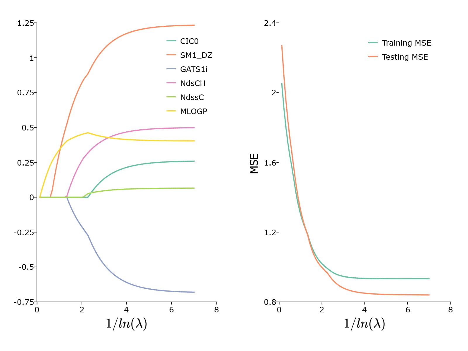
To plot the paths of the coefficients and the MSE, we can use the plotLR() function

test_mse = meanSquaredError(y_test, y_hat);

/*
** Plot results
*/
plotLR(mdl, test_mse);

This results in the following plot:

Remarks¶

Each variable (column of X) is centered to have a mean of 0 and scaled to have unit length, (i.e. the vector 2-norm of each column of X is equal to 1).