The Absolute Basics for Beginners#
Never programmed before? This guide explains the fundamentals from scratch. By the end, you’ll understand what programming is, how GAUSS works, and how to write simple programs.
What is Programming?#
Programming is giving instructions to a computer. The computer follows your instructions exactly—no more, no less.
Think of it like a recipe:
Get 2 eggs
Crack eggs into bowl
Add 1 cup flour
Mix for 2 minutes
A computer program works the same way: step-by-step instructions that the computer executes in order.
The difference: computers need precise instructions in a specific language. GAUSS is that language.
The GAUSS Environment#
When you open GAUSS, you’ll see several panels:
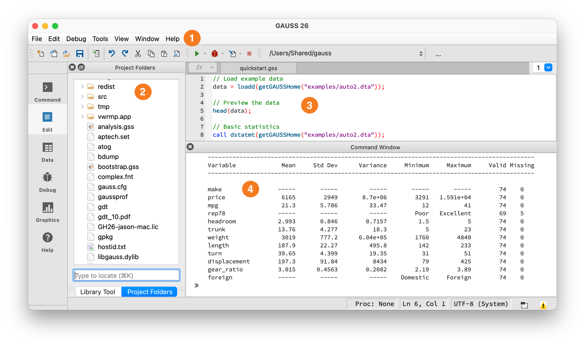
The GAUSS IDE workspace.#
① Toolbar — Shows your current working directory. The Run button (green arrow) is here — click it or press F5 to execute your program.
② Project Folders — Browse and open files in your working directory. Double-click any .e file to open it in the editor.
③ Editor — Write and edit programs here. Save as .e files.
④ Command Window — Output appears here after you run code. You can also type single lines directly at the >> prompt.
For this guide, we’ll start in the Command Window ④. Look for the prompt — it might show >> or just a blinking cursor. That’s where you type.
Two Ways to Run Code#
Way 1: Command Window (interactive)
Click in the Command Window
Type a command
Press Enter
See the result immediately
Good for: testing ideas, quick calculations, learning.
Way 2: Editor (programs)
Type multiple lines of code in the Editor
Save the file (Ctrl+S or Cmd+S) with a
.eextensionClick Run (green arrow) or press F5
See all results in the output area
Good for: real work, saving your analysis, running multiple steps.
For now, use the Command Window. We’ll use the Editor later when programs get longer.
Your First Program#
Click in the Command Window and type this:
print "Hello, World!";
Press Enter. You should see:
Hello, World!
Congratulations—you just ran your first program.
What happened:
printis a command that displays output"Hello, World!"is the text to display (called a “string”);marks the end of the instruction (required in GAUSS)
Variables: Storing Information#
A variable stores a value so you can use it later. Think of it as a labeled box.
x = 5;
print x;
Output:
5.0000000
What happened:
x = 5creates a variable namedxand puts the value 5 in itprint xdisplays whatever is stored inx
You can change what’s in a variable:
x = 5;
print x;

x = 10;
print x;
Output:
5.0000000
10.000000
And use variables in calculations:
x = 5;
y = 3;
z = x + y;
print z;
Output:
8.0000000
Naming rules:
Start with a letter (not a number)
Use letters, numbers, and underscores
Case sensitive (
Xandxare different)Good:
price,total_sales,gdp2020Bad:
2price,total-sales,my variable
Basic Math#
GAUSS handles arithmetic like a calculator:
a = 2 + 3;      // Addition
print a;

b = 10 - 4;     // Subtraction
print b;

c = 5 * 6;      // Multiplication
print c;

d = 20 / 4;     // Division
print d;

e = 2^3;        // Exponent (2 to the power of 3)
print e;
Output:
5.0000000
6.0000000
30.000000
5.0000000
8.0000000
The // starts a comment—text the computer ignores. Comments explain your code to humans.
Order of operations follows standard math rules (PEMDAS):
y = 2 + 3 * 4;      // 3*4 first, then +2 = 14
print y;

z = (2 + 3) * 4;    // Parentheses first = 20
print z;
Output:
14.000000
20.000000
Matrices: GAUSS’s Superpower#
A matrix is a grid of numbers. GAUSS is built around matrices—they’re the core data type.
Create a matrix with braces { }:
// A 2x3 matrix (2 rows, 3 columns)
A = { 1 2 3,
      4 5 6 };
print A;
Output:
1.0000000        2.0000000        3.0000000
4.0000000        5.0000000        6.0000000
Syntax:
{ }encloses the matrixSpaces separate columns
Commas separate rows
;ends the statement
A single number is just a 1x1 matrix:
x = 5;       // This is a 1x1 matrix
y = { 5 };   // Same thing
A column of numbers (a “vector”):
prices = { 10.50,
           12.75,
           9.99,
           15.00 };
print prices;
Matrix dimensions:
A = { 1 2 3, 4 5 6 };
print rows(A);    // Number of rows
print cols(A);    // Number of columns
Output:
2.0000000
3.0000000
Getting Specific Values#
Access elements with square brackets [ ]:
A = { 10 20 30,
      40 50 60 };

print A[1, 1];    // Row 1, Column 1
print A[2, 3];    // Row 2, Column 3
print A[1, .];    // Row 1, all columns
print A[., 2];    // All rows, Column 2
Output:
10.000000
60.000000
       10.000000        20.000000        30.000000
20.000000
50.000000
Key points:
Counting starts at 1 (not 0 like some languages)
Use
.to mean “all” rows or columnsA[1, .]= first rowA[., 1]= first column
Ranges with ::
A = { 1 2 3 4 5,
      6 7 8 9 10 };

print A[1, 2:4];    // Row 1, columns 2 through 4
print A[1:2, 1:2];  // Rows 1-2, columns 1-2
Output:
2.0000000        3.0000000        4.0000000

1.0000000        2.0000000
6.0000000        7.0000000
Math with Matrices#
Add, subtract, multiply, divide—element by element:
A = { 1 2, 3 4 };
B = { 10 20, 30 40 };

C = A + B;      // Add corresponding elements
print C;

D = A .* B;     // Multiply corresponding elements
print D;
Output:
11.000000        22.000000
33.000000        44.000000

10.000000        40.000000
90.000000        160.00000
Important: The . before * means “element-wise.” Without it, * does matrix multiplication (a different operation):
A = { 1 2, 3 4 };
B = { 10 20, 30 40 };

C = A .* B;    // Element-wise: 1*10, 2*20, 3*30, 4*40
print C;

D = A * B;     // Matrix multiply: row-by-column
print D;
Output:
10.000000        40.000000
90.000000        160.00000

70.000000        100.00000
150.00000        220.00000
Scalar operations apply to every element:
A = { 1 2, 3 4 };

B = A + 10;     // Add 10 to every element
print B;

C = A * 2;      // Multiply every element by 2
print C;

D = A^2;        // Square every element
print D;
Output:
11.000000        12.000000
13.000000        14.000000

2.0000000        4.0000000
6.0000000        8.0000000

1.0000000        4.0000000
9.0000000        16.000000
Useful Functions#
GAUSS has hundreds of built-in functions. Here are the most common:
Statistics:
data = { 10, 20, 30, 40, 50 };

print meanc(data);    // Average (mean)
print stdc(data);     // Standard deviation
print sumc(data);     // Sum
print minc(data);     // Minimum
print maxc(data);     // Maximum
Output:
30.000000
15.811388
150.00000
10.000000
50.000000
The c in meanc, sumc etc. means “column”—these work down columns.
Math functions:
print sqrt(16);       // Square root
print ln(2.718);      // Natural log
print exp(1);         // e^1
print abs(-5);        // Absolute value
Output:
4.0000000
0.99989631
2.7182818
5.0000000
Loading Data#
Real analysis uses data from files, not typed-in numbers:
// Load a CSV file
data = loadd("housing.csv");

// See what you loaded
print rows(data) "rows";
print cols(data) "columns";

// View first 5 rows
print data[1:5, .];
How print works: print takes a space-separated list of items and displays them on one line. Here, rows(data) and "rows" are two separate items printed together.
You can also print expressions directly:
a = 3;
b = 4;
print a + b;    // Prints 7
The loadd function reads CSV, Excel, and other formats automatically. It returns a dataframe—a matrix where columns have names. This lets you refer to columns by name (like data[., "price"]) instead of by number.
If the file isn’t in your working directory, use the full path:
data = loadd("/Users/yourname/Documents/data/housing.csv");
Or use GAUSS’s example data:
data = loadd(getGAUSSHome("examples/housing.csv"));
Writing a Simple Analysis#
Now it’s time to use the Editor instead of the Command Window. When you have multiple lines of code, the Editor is easier:
Click in the Editor panel (the large area, usually on the right)
Type or paste the code below
Save the file: File → Save As, name it
housing_analysis.eRun it: Click the green Run button or press F5
Let’s put it together—load data, calculate statistics, show results:
// Load housing data
data = loadd(getGAUSSHome("examples/housing.csv"));

// Extract the price column (loadd creates a dataframe with named columns)
prices = data[., "price"];

// Calculate statistics
avg_price = meanc(prices);
std_price = stdc(prices);
min_price = minc(prices);
max_price = maxc(prices);

// Display results
print "Housing Price Summary";
print "=====================";
print "Average: $" avg_price "thousand";
print "Std Dev: $" std_price "thousand";
print "Minimum: $" min_price "thousand";
print "Maximum: $" max_price "thousand";
Output:
Housing Price Summary
=====================
Average: $       155.33100 thousand
Std Dev: $       101.26221 thousand
Minimum: $       21.000000 thousand
Maximum: $       587.00000 thousand
Common Errors (and How to Fix Them)#
Missing semicolon:
x = 5
print x;
Error: G0008 : Syntax error 'print'
Fix: Add ; after every statement:
x = 5;
print x;
Undefined variable:
print y;
Error: G0025 : Undefined symbol: 'y'
Fix: Make sure you created the variable first:
y = 10;
print y;
File not found:
data = loadd("mydata.csv");
Error: csvRead error: file 'mydata.csv' not found
Fix: Check the filename and use the full path if needed:
data = loadd("/full/path/to/mydata.csv");
Dimension mismatch:
A = { 1 2, 3 4 };
B = { 1, 2, 3 };
C = A * B;
Error: G0036 : Matrix dimensions are incompatible
Fix: Make sure matrices have compatible dimensions for the operation. Here, A is 2x2 and B is 3x1—they can’t be multiplied.
Next Steps#
You now understand:
Variables and basic math
Matrices (creating, indexing, operations)
Loading data
Using functions
Common errors
Ready for more?
GAUSS Quickstart — A faster-paced introduction with more features
Data Management — Working with real datasets
Running Existing Code — If you have code to run
Practice suggestion: Try modifying the housing analysis above to calculate statistics for a different column (like size or beds).