GAUSS Quickstart#
This 10-minute guide gets you writing and running GAUSS code. You’ll learn to create matrices, load data, run a regression, and make a plot.
Prerequisites#
GAUSS installed
Basic familiarity with any programming language (helpful but not required)
Where to type code: Open GAUSS and create a new program file (File → New). Type or paste the examples below, then click the Run button to execute. You can also type single lines in the Command Window at the bottom.
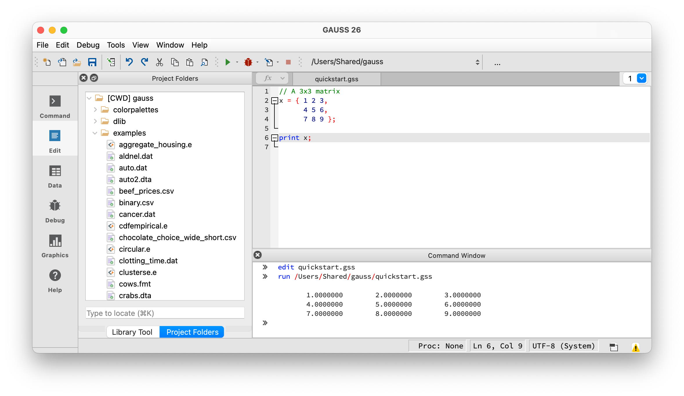
Code goes in the Editor (top right). Output appears in the Command Window (bottom).#
Creating Matrices#
Everything in GAUSS is built on matrices. A dataframe is a matrix with named, typed columns – you get one when you load data with loadd(). We’ll start with plain matrices, then work with dataframes starting in Loading Data below.
Every GAUSS statement ends with a semicolon (;). Lines starting with // are comments.
Create a matrix by listing values in braces, with spaces separating columns and commas separating rows:
// A 3x3 matrix
x = { 1 2 3,
      4 5 6,
      7 8 9 };
print x;
Output:
1.0000000        2.0000000        3.0000000
4.0000000        5.0000000        6.0000000
7.0000000        8.0000000        9.0000000
Create sequences with seqa():
// Start at 1, increment by 1, 5 elements
x = seqa(1, 1, 5);
print x;
Output:
1.0000000
2.0000000
3.0000000
4.0000000
5.0000000
Generate random data with rndn() (standard normal):
// 3 rows, 4 columns of random normals
x = rndn(3, 4);
print x;
Your output will differ since the values are random.
Basic Operations#
GAUSS uses * for matrix multiplication and .* for element-wise multiplication. The same dot-prefix pattern applies to division (./) and exponentiation (.^). Addition and subtraction (+, -) always work element-wise:
// A 5x1 column vector (commas separate rows)
x = { 1, 2, 3, 4, 5 };

// Element-wise square
y = x.^2;

// Horizontal concatenation with ~ (joins columns side by side)
print x~y;
Output:
1.0000000        1.0000000
2.0000000        4.0000000
3.0000000        9.0000000
4.0000000        16.000000
5.0000000        25.000000
Common statistical functions:
x = rndn(100, 3);

print "Column means:";
print meanc(x);

print "Column std devs:";
print stdc(x);

// sumc sums each column; nest it to get the grand total
print "Sum of all elements:";
print sumc(sumc(x));
Loading Data#
Use loadd() to load CSV, Excel, SAS, Stata, or GAUSS datasets:
// Get full path to a dataset included with GAUSS
fname = getGAUSSHome("examples/housing.csv");

// Load the data
data = loadd(fname);

print rows(data) "rows," cols(data) "columns";
Output:
100.00000 rows, 6.0000000 columns
View column names:
print getcolnames(data);
Output:
taxes
 beds
baths
  new
price
 size
Preview the first few rows (the . means “all columns”):
print data[1:5, .];
Output:
    taxes             beds            baths              new            price             size
3104.0000        4.0000000        2.0000000        0.0000000        279.90000        2048.0000
1173.0000        2.0000000        1.0000000        0.0000000        146.50000        912.00000
3076.0000        4.0000000        2.0000000        0.0000000        237.70000        1654.0000
1608.0000        3.0000000        2.0000000        0.0000000        200.00000        2068.0000
1454.0000        3.0000000        3.0000000        0.0000000        159.90000        1477.0000
Running a Regression#
Use olsmt() for OLS regression with a formula string. Inside the formula, ~ separates the dependent variable from the independent variables, and + lists the predictors. (This ~ is unrelated to the concatenation operator — it only has this meaning inside a formula string.)
call discards the return value — use it when you just want the printed report:
// Load the housing dataset
fname = getGAUSSHome("examples/housing.csv");
data = loadd(fname);

// Regress price on beds, baths, and size
call olsmt(data, "price ~ beds + baths + size");
Output:
Ordinary Least Squares
====================================================================================
Valid cases:                      100          Dependent variable:             price
Missing cases:                      0          Deletion method:                 None
Total SS:                    1.02e+06          Degrees of freedom:                96
R-squared:                      0.701          Rbar-squared:                   0.692
Residual SS:                 3.03e+05          Std. err of est:                 56.2
F(3,96):                         75.1          Probability of F:            4.38e-25
====================================================================================
                            Standard                    Prob       Lower       Upper
Variable        Estimate       Error     t-value        >|t|       Bound       Bound
------------------------------------------------------------------------------------

CONSTANT          -27.29      28.241    -0.96634      0.3363     -82.641      28.061
beds             -14.466      10.583     -1.3668     0.17487     -35.209      6.2779
baths             6.8903       13.54     0.50888       0.612     -19.648      33.429
size             0.13043    0.011951      10.914  1.6423e-18     0.10701     0.15386
====================================================================================
The output shows coefficients, standard errors, t-values, p-values, and confidence intervals. House size is the only significant predictor (p < 0.001).
Creating Plots#
GAUSS has built-in plotting functions. Here’s a scatter plot:
// Generate sample data
x = seqa(1, 0.5, 20);
y = 2 + 0.5*x + rndn(20, 1)*0.3;

// Create a scatter plot
plotScatter(x, y);
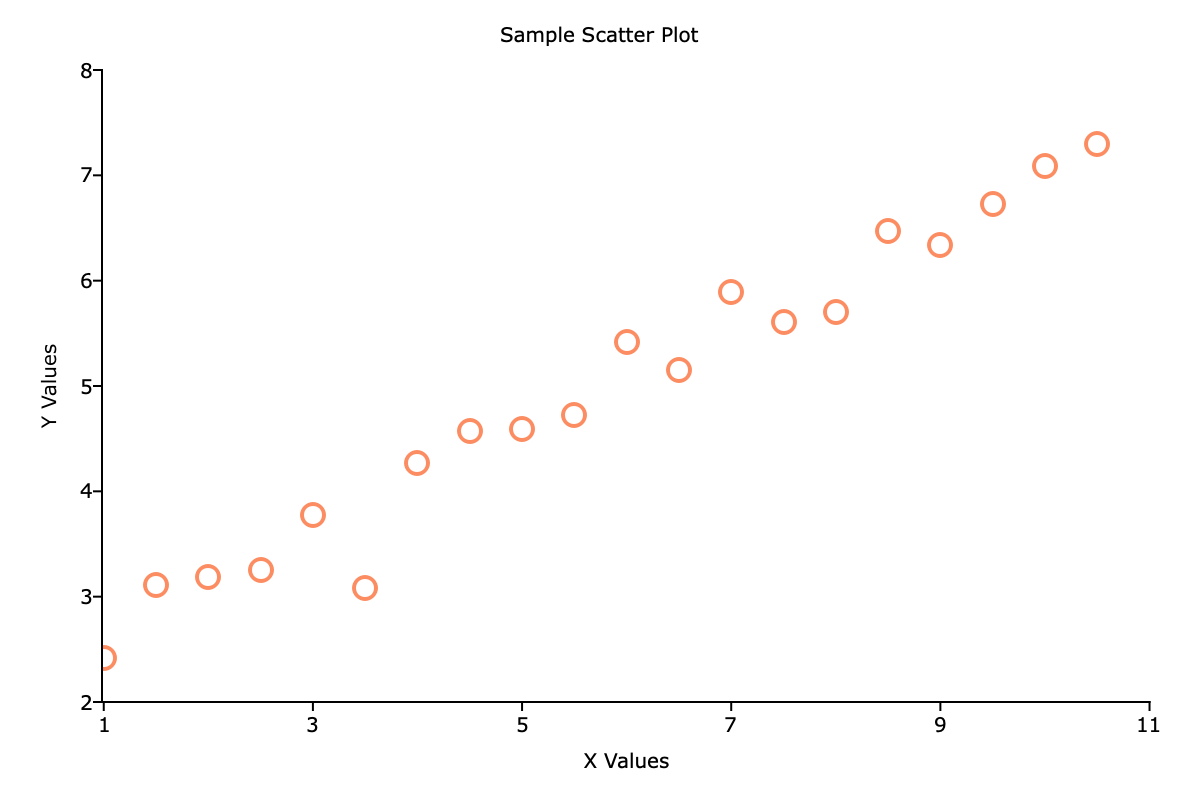
A basic scatter plot#
Customize plots with a plotControl structure. Create one, set options on it with plotSet functions, then pass it to the plot call. The & before the structure name is required so the function can update the settings:
struct plotControl myPlot;
myPlot = plotGetDefaults("scatter");

plotSetTitle(&myPlot, "Housing: Price vs Size");
plotSetXLabel(&myPlot, "Square Feet");
plotSetYLabel(&myPlot, "Price ($000s)");

fname = getGAUSSHome("examples/housing.csv");
data = loadd(fname);

// data[., "size"] selects all rows of the column named "size"
plotScatter(myPlot, data[., "size"], data[., "price"]);
For histograms:
fname = getGAUSSHome("examples/housing.csv");
data = loadd(fname);
plotHist(data[., "price"], 15);
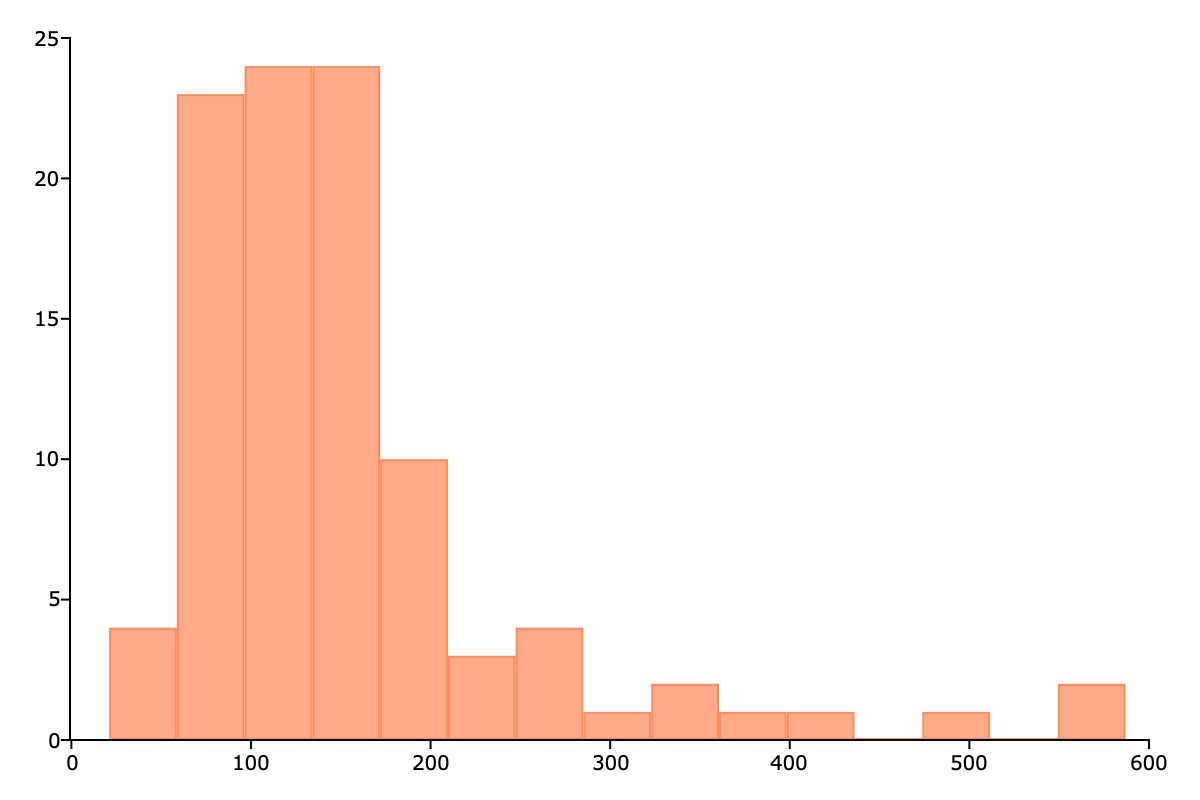
Distribution of housing prices#
Saving Your Work#
Save the most recent plot to a file with plotSave(). The | operator stacks values into a column vector — here it creates a 2x1 width-by-height size:
// Save the last plot as an 800x600 PNG
plotSave("my_scatter.png", 800|600, "px");
Files are saved to your GAUSS working directory (shown at the top of the GAUSS window).
Save data with saved():
// Save as CSV
saved(data, "mydata.csv");

// Save as GAUSS dataset (.gdat preserves column names and types)
saved(data, "mydata.gdat");
What’s Next?#
The Absolute Basics for Beginners — If you’re new to programming
Running Existing Code — If you inherited GAUSS code
Data Management — Loading and transforming data
Command Reference — Full function reference