Introduction to GAUSS for Stata Users

This page provides a basic overview of how common Stata operations can be implemented in GAUSS. It is not meant to serve as a comprehensive GAUSS guide. However, we do provide references for those who wish to explore topics in greater depth.

Data Storage

GAUSS stores data in matrices, string arrays, and dataframes. One of the key differences between data storage in GAUSS and Stata is that GAUSS allows you to store data from multiple sources simultaneously.

In Stata, people are most familiar with working with a single dataset in memory. Stata does allow you to store multiple datasets in memory using specified dataframes but special commands must be used to switch between frames.

Reference	GAUSS	Stata
Data structure	Dataframe or matrix	Data set
Series of data	Column	Variable
Single occurrence	Row	Observation
Missing Values	.	.

What is a GAUSS dataframe?

A GAUSS dataframe is used to store two-dimensional data and allows you to store:

• Data in rows and columns.

• Information about the data type and type-related properties.

• Different variables together, including categorical data, strings, and dates.

Many internal functions are designed to work intelligently with dataframes to use variable names and types for estimation and reporting.

For example, olsmt() will use the information stored in a dataframe during estimation to:

• Properly include dummy variables when categorical independent variables are present.

• Include variable names in output reports.

Variables

Each column of a GAUSS dataframe contains a series of data for a single variable. Variables are stored as strings, numbers, categories, or dates.

In Stata, variables are referenced directly by name.

list mpg

In GAUSS, variables can be referenced by indexing with variable name or by column number. However, we must tell GAUSS which dataframe to look for the variable in.

For example, if the variable mpg is stored in the fourth column of the dataframe auto2 we could use either

auto2[., "mpg"];

or

auto2[., 4];

to reference the variable.

Note

The . indicates to GAUSS that all rows are being indexed. This will be discussed in more detail in the indexing section.

Variable Type	Description	Examples
String	The string data type can contain letters, numbers, and other characters.	Customer names, product names, or book titles.
Number	Analogous to the data stored in GAUSS matrices.	Daily temperatures, real GDP, stock prices.
Categories	Houses discrete variables that capture qualitative data.	Marriage status, performance ratings, transportation modes.
Dates	Houses and displays dates and times.	Purchase date, shipping date, observation date.

Observations

Each row of a GAUSS dataframe contains simultaneous observations of variables. In time series data or panel data , this may correspond to dates of observations. In cross-sectional data, this may correspond to some other identifier such as identification number, observation number, or name.

Rows of data are indexed by row number. For example, if we want to access the data stored in the fourth row we use

auto2[4, .];

Data Input/Output

Constructing a dataframe from values

In Stata, the input statement is used to build datasets from specified values and column names:

input  x y
1 2
3 4
5 6
end

In GAUSS, a dataframe can be created from a manually entered matrix and variable names using the asDF() procedure:

// Create a 3 x 2 matrix
mat = { 1 2,
        3 4,
        5 6 };

// Convert matrix to a dataframe
// and name the first column "X"
// and the second column "Y"
df = asDF(mat, "X", "Y");

Reading external datasets

GAUSS can directly read and load data from most data formats, including:

• CSV

• Excel (XLS, XLSX)

• HDF 5

• GAUSS matrices (FMT)

• GAUSS datasets (DAT)

• Stata datasets (DTA)

• SAS datasets (SAS7BDAT, SAS7BCAT)

• SPSS datasets (SAV)

In Stata, the import command is used to import non-Stata datasets. Additional information must be provided to specify what type of file is being imported.

import excel "nba_ht_wt.xls", clear

Alternatively, the tips2.csv dataset is loaded into Stata using the import delimited command

import delimited "tips2.csv", clear

Note

The use of the clear option is necessary in Stata if the data is already loaded into the workspace. In GAUSS, this is not necessary because multiple data sets can be loaded into the work space simultaneously.

In GAUSS, all data files are usually loaded using the loadd() procedure. For example, consider loading the auto2.dta dataset:

// Load all variables from the file 'auto2.dta'
// using their default types
auto2 = loadd(getGAUSSHome $+ "examples/auto2.dta");

This loads all the variables in the dataset and auto-detects their type.

Sometimes, you may need to specify the type and/or variables that you wish to load. This is done using a formula string:

For example, let’s consider loading the nba_ht_wt.xls file in GAUSS

// Create filename
fname = getGAUSSHome $+ "examples/nba_ht_wt.xls";

// Load the file 'nba_ht_wt.xls'
// using a formula string to select variables
// and specify variable types
nba_ht_wt = loadd(fname, "str(Player) + cat(Pos) + Height + Weight + str(School)");

Similarly, the tips2.csv data file:

// Create filename
fname = getGAUSSHome $+ "examples/tips2.csv";

// Load the file 'tips2.csv'
// using a formula string to select variables
// and specify variable types
tips2 = loadd(fname, "id + total_bill + tip + cat(sex) + cat(time)");

Note

The getGAUSSHome() function is a convenience function that returns the full path to the GAUSS home directory.

Formula strings accept a number of operators and keywords which allow you to:

• Specify variable types.

• Perform data transformations.

Operator	Purpose
.	Represents all variables.
+	Adds a variable.
-	Removes a variable.
1	Represents an intercept term.
*	Adds an interaction term and includes both original variables.
:	Adds an interaction term between two variables but does not include either of the original variables.

Keyword	Purpose
cat	Load a variable as a categorical column.
date	Load a variable as a date column.
str	Load a variable as a string column.
$	Indicate that a variable is stored in the file as a string as should be passed to the keyword or procedure as a string column.

The GAUSS Data Management guide provides a complete guide to Programmatic Data Import.

Interactively loading data

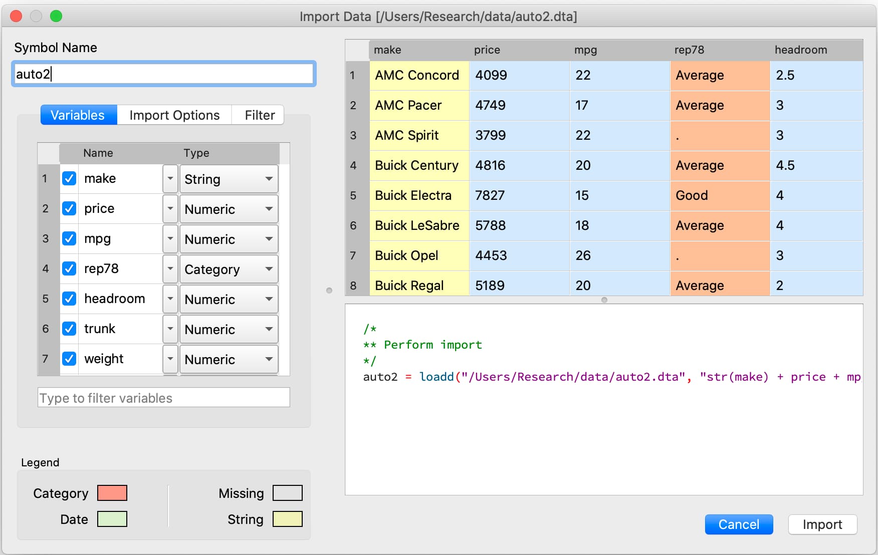
The GAUSS Data Import window is a completely interactive environment for loading data and performing preliminary data cleaning. It can be used to:

• Select variables and change types.

• Select observation by range or logic filtering.

• Manage date formats and category labels.

• Preview data.

The Data Import window offers a data import experience similar to Stata’s menu driven data import. Like Stata, the GAUSS Data Import window auto-generates code that can be reused.

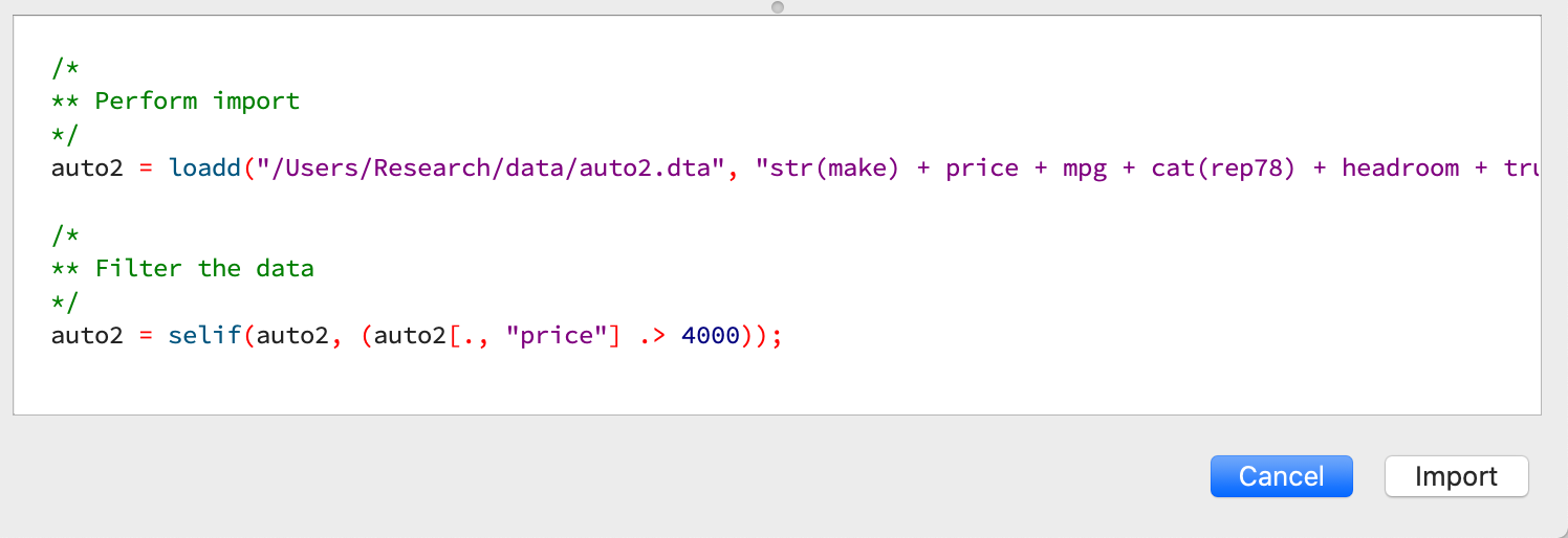
You can open the Data Import window in three ways:

• Select File > Import Data from the main GAUSS menu bar.

• From the Project Folders window:

  • Double-click on the name of the data file.

  • Right-click the file and select Import Data.

A complete guide to interactively loading data is available in the GAUSS Data Management guide.

Viewing Data

Data can be viewed in GAUSS a number of ways:

• Using the GAUSS Data Editor.

• Opening a floating Symbols Editor window using Ctrl+E.

• Printing data to the Command Window.

For a quick preview, portions of a dataframe can be printed directly to screen using indexing. For example, the first five rows the auto2 dataframe can be printed to screen by entering

auto2[1:5, .];

This is equivalent to using the list command in Stata

list 1/5

If we only wanted to view the first five rows of the variable mpg from the auto2 dataframe, we would use

auto2[1:5, "mpg"];

which is equivalent to

list mpg 1/5

In GAUSS, you can also preview the beginning or end of your data using the head() or tail() functions, respectively.

For example, to view the first five rows of make, price, and mpg in the dataframe auto2:

head(auto2[., "make" "price" "mpg"]);

This prints

         make            price              mpg
  AMC Concord        4099.0000        22.000000
    AMC Pacer        4749.0000        17.000000
   AMC Spirit        3799.0000        22.000000
Buick Century        4816.0000        20.000000
Buick Electra        7827.0000        15.000000

We can include an optional input to indicate how many rows to include. A positive number specifies how many rows to print. For example, to print the first ten rows:

head(auto2[., "make" "price" "mpg"], 10);

This prints the first ten rows:

         make          price              mpg
    AMC Pacer      4749.0000        17.000000
Buick Century      4816.0000        20.000000
Buick Electra      7827.0000        15.000000
Buick LeSabre      5788.0000        18.000000
   Buick Opel      4453.0000        26.000000
  Buick Regal      5189.0000        20.000000
Buick Riviera      10372.000        16.000000
Buick Skylark      4082.0000        19.000000

A negative number indicates how many rows to skip before beginning printing. For example, to print everything after the first 10 rows of data:

head(auto2[., "make" "price" "mpg"], -10);

Data Operations

Indexing matrices and dataframes

GAUSS uses square brackets [] for indexing matrices. The indices are listed row first, then column, with a comma separating the two. For example, to index the element in the 3rd row and 7th column of the matrix x, we use:

x[3, 7];

To select a range of columns or rows with numeric indices, GAUSS uses the : operator:

x[3:6, 7];

GAUSS also allows you to use variable names in a dataframe for indexing. As an example, if we want to access the 3rd observation of the variable mpg in the auto2 dataframe, we use:

auto2[3, "mpg"];

You can also select multiple variables using a space separated list:

auto2[3, "mpg" "make"];

Finally, GAUSS allows you index an entire column or row using the . operator. For example, to see all observations of the variable mpg in the auto2 dataframe, we use:

auto2[., "mpg"];

Operations on variables

In Stata, generate and replace are required to either transform existing variables or generate new variables using existing variables:

replace total_bill = total_bill - 2
generate new_bill  = total_bill / 2

In GAUSS, these operations are performed using operators. For example, GAUSS uses:

• The - operator to subtract values.

• The / operator to divide values.

• The = to assign the new values to a storage location.

• The ~ to add new columns to a matrix or dataframe.

// Subtract 2 from all observations of the
// variable 'total_bill' in the 'tips2' dataframe
tips2[., "total_bill"] = tips2[., "total_bill"] - 2;

// Divide all observations of the variable
// 'total_bill' in the 'tips2' dataframe by 2
tips2[., "total_bill"] = tips2[., "total_bill"] / 2;

// Divide all observations of the variable
// 'total_bill' in the 'tips2' dataframe by 2
// and generate 'new_bill'
tips2 = tips2 ~ dfname(tips2[.,"total_bill"] / 2, "new_bill");

Matrix operations

GAUSS is a matrix based language and matrix operations play a fundamental role in GAUSS computations.

Common Matrix Operators

Description	GAUSS	Stata
Matrix multiply	z = x * y;	matrix z = x*y
Solve system of linear equations	b = y / x;	matrix b = y*inv(x)
Kronecker product	z = x .*. y;	matrix z = x#y
Matrix transpose	z = x';	matrix z = x’

When dealing with matrices, it is important to distinguish matrix operations from element-by-element operations. In Stata, element-by-element operations are specified with a colon :. In GAUSS, element-by-element operations are specified by a dot ..

Element-by-element (ExE) Operators

Description	GAUSS	Stata
Element-by-element multiply	z = x .* y;	matrix z = x:*y
Element-by-element divide	z = y ./ x;	matrix z = y:/x
Element-by-element exponentiation	z = x .^ y;	matrix z = x:^y
Element-by-element addition	z = x + y;	matrix z = x + y
Element-by-element subtraction	z = x - y;	matrix z = x - y

For a more in depth look at how matrix operation works in GAUSS you may want to review our blogs:

• GAUSS Basics 3: Intro to Matrices

• GAUSS Basics 4: Matrix Operations

• GAUSS Basics 5: Element-by-Element Conformability

Filtering

In Stata, data is filtered using an if clause when using other commands. For example, to keep all observations where total_bill is greater than 10 we use:

keep if total_bill > 10

In GAUSS this can be done interactively with the Data Management Tool:

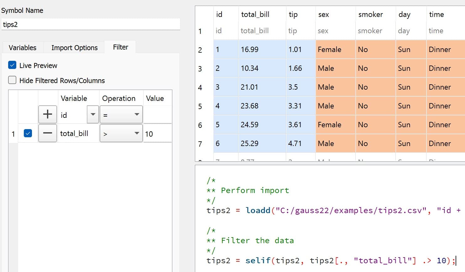
Programmatically this is done using the selif() procedure:

// Select observations from the tips2 dataframe
// where the total_bill variable is greater than 10
tips2 = selif(tips2, tips2[., "total_bill"] .> 10);

More information about filtering data can be found in:

• The Interactive Data Cleaning section of the Data Management Guide.

• Preparing and Cleaning FRED data in GAUSS

• Getting to Know Your Data with GAUSS 22

Selection of data

Stata allows you to select, drop, or rename columns using command line keywords:

keep sex total_bill tip

drop sex

rename total_bill total_bill_2

In GAUSS, the same can be done using the Data Management pane.

To open the Data Management pane:

1. Double-click the name of the dataframe in the Symbols window on the Data page.

2. Click the Manage button with the cog icon on the top right of the open Symbol Editor window.

Select columns from a dataframe

Columns can be selected or removed from the dataframe using the Variables list.

• If a variable has a check box next to the name of the variables it is included in the dataframe.

• To clear the variable from the dataframe clear the check box next to the variable name.

These changes will not be made until you click Apply.

Changing variable names

Variable names can also be changes from the Variables list.

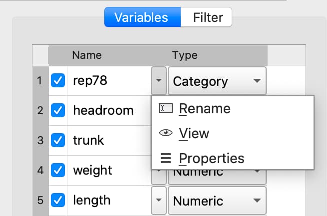
1. Double-click the dataframe you want to modify in the Symbols pane of the Data page.

2. Click the Manage button at the top right of the open Symbol Editor.

3. Click downward pointing triangle button to the right of the name of the variable name you want to change and select Rename.

4. Enter the new name in the Name text box.

These changes will not be made until you click Apply.

GAUSS also offers programmatic options for selecting data and changing variable names:

// Keep only 'total_bill' 'tip' and 'sex'
tips2 = tips2[., "total_bill" "tip" "sex"];

// Drop sex variable
tips2 = delcols(tips2, "sex");

// Rename variable 'total_bill' to 'total_bill_2'
tips2 = dfname(tips2, "total_bill_2", "total_bill");

Sorting

In Stata the sort command is used for sorting data:

sort sex total_bill

In GAUSS, this is done using sortc().

We can accomplish the same sorting as the Stata line above using:

// Sort the 'tips2' dataframe based
// on 'sex' and 'total_bill' variables
tips2 = sortc(tips2, "sex" $| "total_bill");

Date Functionality

GAUSS dataframes include a date data type which makes it convenient to read, format, and use dates in analysis.

Date variables can be loaded interactively using the Data Import window or programmatically using loadd() and the date keyword.

Creating usable dates from raw data

In Stata, dates are most often imported as strings from raw data. They must then be converted to usable date types using the date() function and a readable format is set using format.

For example, when the yellowstone.csv dataset is imported into Stata, the variable date is a string variable The date variable must be converted to a date type:

generate date_var = date(date, "YMD");

and the viewing format should be set

format date_var %d.

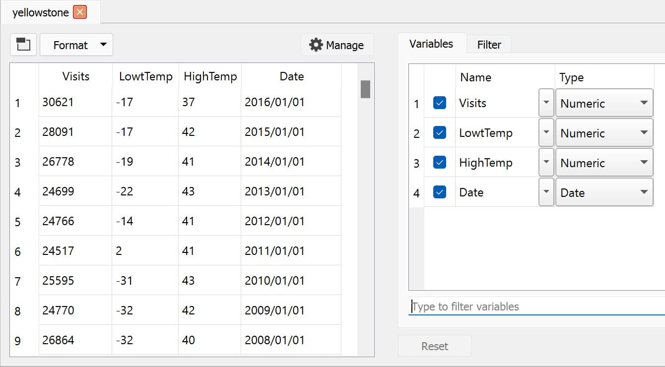
In GAUSS, dates can be directly read in as date variables using the loadd() procedure and the date keyword. The loadd() procedure automatically detects common date formats and doesn’t require a format specification unless a custom format is being used in the raw data:

// Create filename
fname = getGAUSSHome $+ "examples/yellowstone.csv";

// Load the variable Visits, LowtTep, HighTemp and Date
// from the file 'yellowstone.csv'
yellowstone = loadd(fname, "Visits + LowtTemp + HighTemp + date($Date)");

Creating dates from existing strings

The GAUSS asDate() procedure works similarly to the Stata date() function and can be used to convert strings to dataframe dates.

For example, suppose we want to convert the string "2002-10-01" to a date in Stata:

generate date_var = date("2002-10-01", "YMD")

When we do this in Stata the data is displayed in the date numeric format and we have to use the format command to change the display format:

format date_var %d

In GAUSS, this is done using the asDate() procedure:

// Convert string date '2002-10-01'
// to a date variable
date_var = asDate("2002-10-01");

The asDate() procedure automatically recognizes dates in the format "YYYY-MM-DD HH:MM:SS". However, if the date is in a different format, a format string can be used:

// Convert string date '10/01/2002'
// to a date variable
date_var = asDate("10/01/2002", "%d/%m/%Y");

Changing the display format

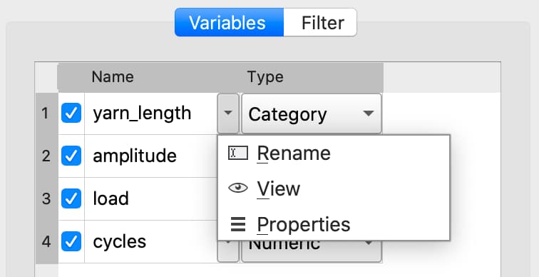
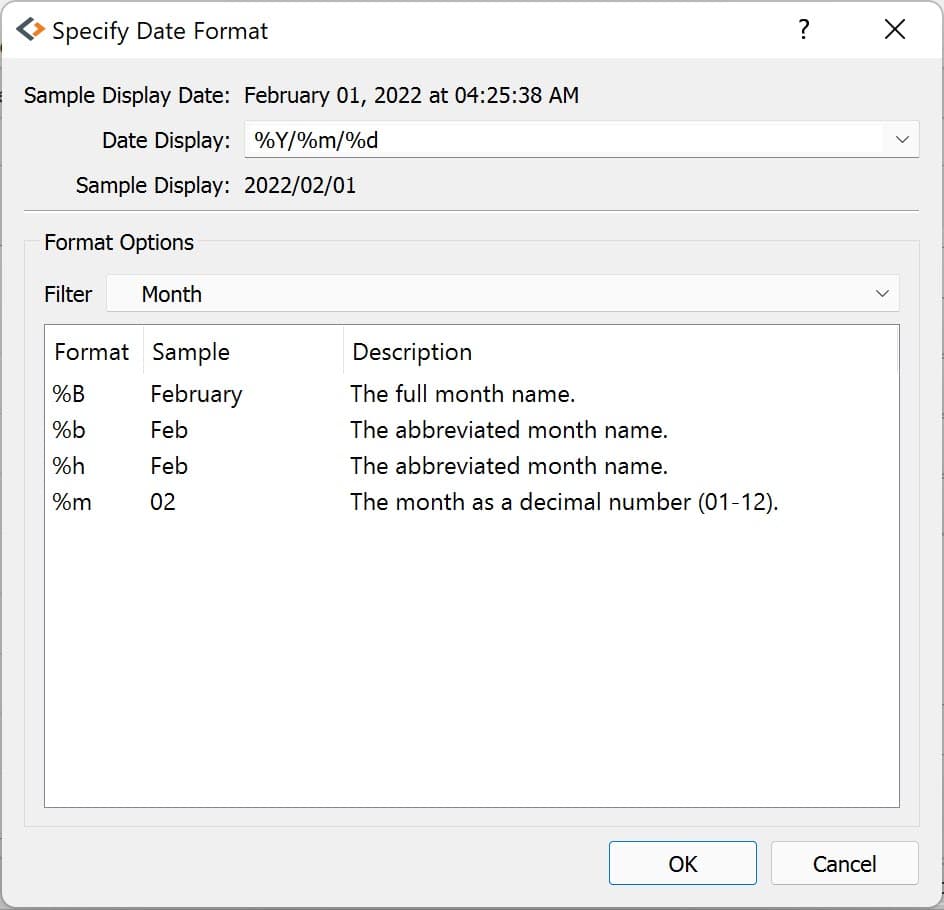
Once a date variable has been imported or created, the display format can be specified interactively using the GAUSS Data Management Tool.

The Specify Date Format dialog is accessed by selecting Properties from the variable’s dropdown:

If the variable is a date variable, the Specify Date Format window will open:

Dates can be managed programmatically using asDate():

// Convert 'Date' variable from string variable
// to date variable
yellowstone =  asdate(yellowstone, "%b-%d-%Y", "Date");

String Processing

Finding the length of a string

The strlen() and ustrlen() functions are used in Stata to find the length of strings:

generate strlen_time = strlen(time)
generate ustrlen_time = ustrlen(time)

GAUSS also uses a strlen() procedure to find string lengths:

// Find length of all observations
// of the variable 'time' in
// the 'tips2' dataframe
strlen_time = strlen(tips2[., "time"]);

Finding the position of a substring

Finding the position of strings can be useful for data searching and cleaning. In Stata, the strpos() function allows you to find the location of a specified substring within another string:

generate str_position = strpos(sex, "ale")

In GAUSS, this is done using the strindx() or strrindx() procedures. The strindx() procedure searches from the beginning of the string and the strrindx() procedure searches from the end of the string.

The functions require two inputs:

• where (string or scalar) – the data to be searched.

• what (string or scalar) – the substring to be searched for in where.

For example consider the sex variable in the tips2 dataframe. The first ten observations are:

tips2[1:10, "sex"];

           sex
        Female
          Male
          Male
          Male
        Female
          Male
          Male
          Male
          Male
          Male

// Find the location of the substring 'ale'
// in the variable 'sex' in the 'tips2' dataframe
str_pos = strindx(tips2[., "sex"], "ale");

// Display the first 10 observations of
// all variables in 'str_pos'
str_pos[1:10, .];

The printed result is:

4.0000000
2.0000000
2.0000000
2.0000000
4.0000000
2.0000000
2.0000000
2.0000000
2.0000000
2.0000000

Extracting a substring by position

In Stata, the substr() function is used to extract substrings from a string. The substr() function uses position and string length to specify which substring to extract:

generate short_sex = substr(sex, 1, 1)

The same thing can be done in GAUSS using the strsect():

// Extract first letter from
// the variable 'sex' in the
// 'tips2' dataframe
short_sex = strsect(tips2[., "sex"], 1, 1);
short_sex[1:5, .];

The printed result is:

sex
  F
  M
  M
  M
  F

Extracting words

Stata allows you to extract the nth word from a string using the word() function. For example, to consider if we wish to separate the first and last names from a name into two variables.

clear
input str20 name
"John Smith"
"Jane Cook"
end

generate first_name = word(name, 1)
generate last_name = word(name, -1)

While GAUSS doesn’t have an exactly analogous function, this can be done fairly easily using the strsplit() procedure.

The strsplit() procedure splits the string using an optional specified separator. If no separator is provided, strsplit() separates strings based on spaces.

For example:

// Generate string array of names
string name = { "John Smith", "Jane Cook" };

// Split into two strings
// and name variables 'first_name' and 'last_name'
name_split = asDF(strsplit(name), "first_name", "last_name");

This creates the name_split dataframe:

first_name        last_name
      John            Smith
      Jane             Cook

If the original name data has first, middle, and last names, all separated by spaces, then strsplit() will split the strings into three columns:

// Generate string array of names
string full_name = { "John Robert Smith", "Jane Elizabeth Cook" };

// Split into three strings
// and name variables 'first_name', 'middle_name', and 'last_name'
name_split = asDF(strsplit(full_name), "first_name", "middle_name", "last_name");

Now the name_split variable contains three variables:

first_name      middle_name        last_name
      John           Robert            Smith
      Jane        Elizabeth             Cook

Finally, suppose our names are separated by a comma and a space, instead of a space:

// Generate string array of names
string name = { "Smith,John", "Cook,Jane" };

// Split into two strings using ', ' as a separator
// and name variables 'last_name' and 'first_name'
name_split = asDF(strsplit(name, ", "), "last_name", "first_name");

Now our name_split variable is:

last_name       first_name
    Smith             John
     Cook             Jane

Changing case

GAUSS uses the upper() and lower() procedures to change all letters in strings to uppercase and lowercase, respectively.

For example:

// Change time variable in 'tips2' to all uppercase
tips2[., "time"] = upper(tips2[., "time"]);

// Change sex variable in 'tips2' to all lowercase
tips2[., "sex"] = lower(tips2[., "sex"]);

This compares to the strupper() and strlower() functions in Stata, which change all letters in a string to uppercase and lowercase, respectively.

generate upper_time = strupper(time)
generate lower_sex = strlower(sex)

Missing values

Missing values are represented by the same dot notation, ., in both Stata and GAUSS.

This notation can be used for filtering data Stata:

* Keep missing values
list if value_x == .

* Keep non-missing values
list if value_x != .

In GAUSS missing values can be created with a statement or using the error() function:

// Keep missing values
mss = { . };
data = selif(data, data[., "x"] .== mss));

// Keep non-missing values
data = selif(data, data[., "x"] .!= error(0));

Counting missing values

In Stata, missing values in individual variables can be counted using the count command. This command works with a logical statement specifying what condition is to be counted:

count if rep78 == .

In GAUSS, missing values can be counted using the counts() function and error(0):

counts(auto2[., "rep78"], error(0));

This finds how many missing values there are in the rep78 variable, found in the auto2 dataframe:

5.0000000

Alternatively, missing values are counted as part of the descriptive statistics using dstatmt():

// Get descriptive statistics
call dstatmt(auto2);

This returns

---------------------------------------------------------------------------------------------
Variable             Mean     Std Dev      Variance     Minimum     Maximum     Valid Missing
---------------------------------------------------------------------------------------------
make                -----       -----         -----       -----       -----        74    0
price                6165        2949       8.7e+06        3291   1.591e+04        74    0
mpg                  21.3       5.786         33.47          12          41        74    0
rep78               -----       -----         -----        Poor   Excellent        69    5
headroom            2.993       0.846        0.7157         1.5           5        74    0
trunk               13.76       4.277          18.3           5          23        74    0
weight               3019       777.2      6.04e+05        1760        4840        74    0
length              187.9       22.27         495.8         142         233        74    0
turn                39.65       4.399         19.35          31          51        74    0
displacement        197.3       91.84          8434          79         425        74    0
gear_ratio          3.015      0.4563        0.2082        2.19        3.89        74    0
foreign             -----       -----         -----    Domestic     Foreign        74    0

Removing missing values

GAUSS provides two options for removing missing values from a matrix:

• The packr() procedure removes all rows from a matrix that contain any missing values.

• The delif() procedure removes all rows which meet a particular condition.

// Create matrix
a = { 1 .,
      . 4,
      5 6 };

// Remove all rows with a missing value
print packr(a);

will return

5 6

Conversely

// Create matrix
a = { 1 .,
      . 4,
      5 6 };

// Remove all rows with a missing value
// in the second column
print delif(a, a[., 2] .== error(0));

will only delete rows with a missing value in the second column

. 4
5 6

Replacing missing values

GAUSS also provides two functions for replacing missing values:

• The missrv() function.

• The impute() function.

The missrv() function replaces all missing values in a matrix with a user-specified value

// Create matrix
a = { 1 .,
      . 4,
      5 6 };

// Replace all missing values with -999
print missrv(a, -999);

returns

   1 -999
-999    4
   5    6

This is similar to using the replace variable in Stata

replace a = -999 if a >= .

The impute() procedure replaces missing values in the columns of a matrix using a specified imputation method. The procedure offers six potential methods for imputation:

• "mean" - replaces missing values with the mean of the column.

• "median" - replaces missing values with the median of the column.

• "mode" - replace missing values with the mode of the column.

• "pmm" - replaces missing values using predictive mean matching.

• "lrd" - replaces missing values using local residual draws.

• "predict" - replaces missing values using linear regression prediction.

More details about dealing with missing values are available in:

• The Introduction to Handling Missing Values blog.

• The Data Cleaning section of the GAUSS Data Management Guide.

Merging

In Stata merging:

• Is performed using the merge command.

• Is done using a dataset in memory and a data file on disk.

• Keeps all data from the data in memory and the using data.

• Creates a _merge variable indicating if the data point from the original data, the using data, or the intersection of the two.

• Allows for one-to-one, one-to-many, many-to-one, and many-to-many joining operations.

In GAUSS merging:

• Is done using the outerJoin() or innerJoin() procedures.

• Is done completely with data in memory.

• The innerJoin() function only keeps matching observations.

• The outerJoin() function keeps observations either from both data sources or the left-hand data source.

• Allows for one-to-one, one-to-many, many-to-one, and many-to-many joining operations.

As a first example, let’s consider two dataframes. The first contains ID and Age:

    ID      Age
  John       22
  Mary       18
 Susan       34
Connie       45

The second contains ID and Occupation:

   ID      Occupation
 John         Teacher
 Mary         Surgeon
Susan       Developer
Tyler           Nurse

In Stata, we merge these using merge():

* Create and save the age dataset
clear
input str10 ID
John Doe
Mary Jane
Susan Smith
Connie Lee
end

input age
22
18
34
45
end
save df1.dta

* Now create occupation data
* and keep in memory
clear
input str10 ID
John
Mary
Susan
Tyler
end

input str10 occupation
Teacher
Surgeon
Developer
Nurse
end

merge 1:1 ID using df1

We can do the same in GAUSS using outerJoin():

// Create ID strings
string ID1 = { "John", "Mary", "Susan", "Connie" };
string ID2 = { "John", "Mary", "Susan", "Tyler" };

// Create age vector
age = { 22, 18, 34, 45 };

// Create occupation string
string Occupation = { "Teacher", "Surgeon", "Developer", "Nurse" };

// Create first df
df1 = asDF(ID1, "ID") ~ asDF(age, "Age");

// Create second df
df2 = asDF(ID2, "ID") ~ asDF(Occupation, "Occupation");

// Merge dataframes
df3 = outerJoin(df2, "ID", df1, "ID", "full");

The df3 dataframe contains:

    ID       Occupation              Age
  John          Teacher        22.000000
  Mary          Surgeon        18.000000
 Susan        Developer        34.000000
 Tyler            Nurse                .
Connie                .        45.000000

The df3 dataframe contains all observations from both the df1 and df2 dataframes, even if they aren’t matched, because we included the "full" option.

If we just wanted to keep the matches to the keys from the df2 dataframe we would exclude the "full" option:

// Merge dataframes
df3 = outerJoin(df2, "ID", df1, "ID");

Now df3 includes:

   ID       Occupation              Age
 John          Teacher        22.000000
 Mary          Surgeon        18.000000
Susan        Developer        34.000000
Tyler            Nurse                .