Introduction to GAUSS for EViews Users#
This guide helps EViews users do the same things in GAUSS. If you’re comfortable with workfiles, VAR models, IRFs, and ARIMA estimation, you’ll find equivalent tools in GAUSS – with more flexibility for custom models and reproducible workflows.
Note
This guide is written for GAUSS 26. Time series functions (ARIMA, VAR, GARCH) require the TSMT add-on.
How GAUSS Differs from EViews#
Your analysis is code. EViews blends GUI dialogs, command window entries, and program files. In GAUSS, your entire workflow is a program file – reproducible, version-controlled, and shareable. No clicking through dialogs to re-estimate.
No workfile – load data directly. EViews requires creating a workfile first, then importing series into it. GAUSS loads data directly into a dataframe with
loadd()– no workfile setup step.Multiple datasets at once. EViews ties your analysis to one workfile at a time. GAUSS can hold many datasets in memory simultaneously.
Results in structures, not object views. EViews stores results in “equation” and “VAR” objects that you view in windows. GAUSS returns results in structures with named members (
out.b,out.sigma) that you access in code.Full programming language. EViews handles loops and basic logic. GAUSS is a complete matrix programming language – you can write custom estimators, simulation studies, and bootstrap procedures.
Where to type code:
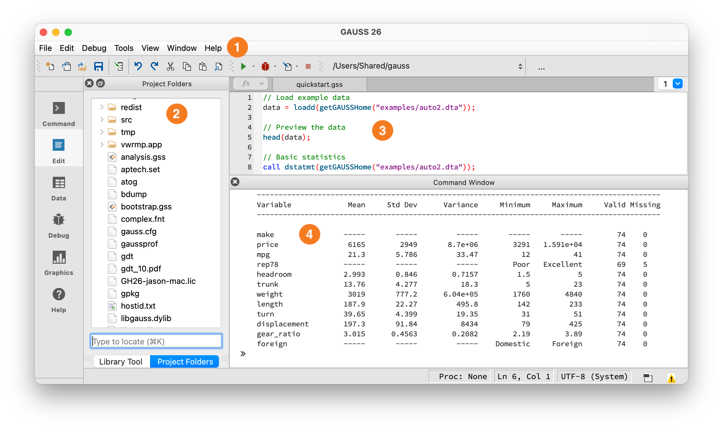
The GAUSS IDE workspace.#
① Toolbar — Shows your current working directory and the Run button (green arrow). Click it or press F5 to execute. ② Project Folders — File browser, similar to EViews’ Workfile contents. ③ Editor — Write programs here, similar to EViews’ program editor. ④ Command Window — Output appears here, similar to EViews’ output window. You can also type single lines at the >> prompt.
Debugging: Errors appear in the Output window with a line number – click it to jump to the error. Use the Variables panel (View > Variables) to inspect values at runtime. You can set breakpoints by clicking in the left margin of the editor, then step through code with the Debug menu. For quick debugging, insert print varname; statements.
Key Syntax Differences#
Feature |
EViews |
GAUSS |
|---|---|---|
Statement end |
Newline |
Required |
Indexing |
1-based (series obs) |
1-based |
String quotes |
|
|
Assignment |
|
|
All rows/cols |
(implicit in series) |
|
Comments |
|
|
String concat |
|
|
String equality |
|
|
Operators#
Matrix vs element-wise multiplication:
// GAUSS
A * B;            // Matrix multiplication
A .* B;           // Element-wise multiplication
A .^ 2;           // Element-wise power
A ./ B;           // Element-wise division
A';               // Transpose
Warning
``*`` is matrix multiplication in GAUSS. EViews handles this behind the scenes. In GAUSS, A * B is matrix multiplication and A .* B is element-wise. Using the wrong one produces wrong results silently.
Comparison operators have two forms. Without a dot, A > 0 returns a scalar – true only if ALL elements satisfy the condition. With a dot, A .> 0 tests each element individually:
// GAUSS
A .> 0;           // Element-wise: returns 1/0 for each element
A .== B;          // Element-wise equality
A .and B;         // Element-wise AND
A .or B;          // Element-wise OR
Warning
A > 0 is true only if every element is positive (like EViews’s @all). A .> 0 tests each element. Both forms exist for: >/.>, </.<, >=/.>=, <=/.<=, ==/.==, !=/.!=.
Concatenation#
// GAUSS
A ~ B;            // Horizontal concatenation (tilde)
A | B;            // Vertical concatenation (pipe)
a $+ b;           // String concatenation
Warning
``|`` is vertical concatenation, not logical OR. condition1 | condition2 stacks two vectors vertically. Use .or for logical OR and .and for logical AND.
For string arrays, use $~ (horizontal) and $| (vertical): "Domestic" $| "Foreign" creates a 2x1 string array.
String operators use the ``$`` prefix. In EViews, + concatenates strings and = compares them. In GAUSS: $+ (concatenation), $== (equality), $~ (horizontal join), $| (vertical join).
Indexing#
EViews manages series by name within a workfile. In GAUSS, you index dataframes directly by row and column:
// GAUSS
data = loadd("gdp_data.xlsx");

data[., "gdp"];           // Column by name (dot = all rows)
data[., "gdp" "cpi"];     // Multiple columns (space-separated names)
data[., 1];               // Column by position
data[1, 1];               // First row, first column
data[1:10, .];            // Rows 1 through 10 (inclusive)
data[rows(data), .];      // Last row (no negative indexing)
Key points:
GAUSS uses
.for “all rows” or “all columns”Slices are inclusive:
data[1:5, .]gets rows 1 through 5No negative indexing. Use
rows(data)for the last row.
Note
Most examples below use the auto2 dataset bundled with GAUSS. To run them, load it first:
auto2 = loadd(getGAUSSHome("examples/auto2.dta"));
Data: Workfiles vs. Dataframes#
In EViews, you create a workfile and import series:
' EViews
wfcreate q 1960Q1 2020Q4
import "gdp_data.xlsx"
In GAUSS, you load data directly into a dataframe – no workfile setup:
// GAUSS - one function reads CSV, Excel, Stata, SAS, SPSS, HDF5
data = loadd("gdp_data.xlsx");

// Check what you loaded
print getcolnames(data)';      // Column names
print rows(data) "observations";
head(data);                     // First 5 rows (like EViews's spreadsheet view)
Loading specific variables uses a formula string with +:
// Load only these variables
data = loadd("macro_data.csv", "gdp + cpi + unrate");

// Load all variables except one
data = loadd("macro_data.csv", ". -date_str");
Accessing variables:
' EViews - reference by name
show gdp
// GAUSS - index by column name
gdp = data[., "gdp"];
Creating new variables:
' EViews
series gdp_growth = dlog(gdp)
series lgdp = log(gdp)
// GAUSS - use lagn() for lags, ln() for natural log
lgdp = ln(data[., "gdp"]);
gdp_growth = lgdp - lagn(lgdp, 1);    // lagn fills the first obs with missing
Warning
log vs ln: EViews’s log() is the natural logarithm. GAUSS’s log() is base 10. Use ln() in GAUSS. Forgetting this will silently corrupt every model that uses logged variables.
Generating lags and differences:
' EViews
series y_lag1 = y(-1)
series y_lag2 = y(-2)
series dy = d(y)
// GAUSS
y_lag1 = lagn(y, 1);                  // Lag 1 (first obs becomes missing)
y_lag2 = lagn(y, 2);                  // Lag 2 (first two obs become missing)
dy = y - lagn(y, 1);                  // First difference
dlog_y = ln(y) - lagn(ln(y), 1);      // Log difference (like EViews's dlog)
Data Import/Export#
// GAUSS - loadd handles all formats
data = loadd("data.csv");
data = loadd("data.dta");             // Stata
data = loadd("data.sas7bdat");        // SAS
data = loadd("data.xlsx");            // Excel

// Export
saved(data, "output.csv");
saved(data, "output.xlsx");
Formula string quick reference: GAUSS uses formula strings in several contexts:
Data Manipulation#
' EViews
smpl if foreign = 0
sort mpg
// GAUSS
domestic = selif(auto2, auto2[., "foreign"] .== 0);   // Filter rows
sorted = sortc(auto2, "mpg");                          // Sort by column
Warning
GAUSS does not support boolean indexing. Use selif() to filter rows: selif(df, condition). Passing a boolean vector to brackets will not filter – it interprets the 0s and 1s as row numbers.
Common operations:
EViews |
GAUSS |
|---|---|
|
|
|
|
|
|
|
|
(manual in EViews) |
|
Missing Values#
EViews handles missing values within the workfile automatically. In GAUSS, you manage them explicitly:
' EViews
series y_clean = @nan(y, 0)
smpl if y <> NA
// GAUSS
miss();                       // Creates a missing value (like EViews's NA)
ismiss(x);                    // Returns 1 if ANY element is missing (scalar)
x .== miss();                 // Element-wise check (returns 1/0 vector)
packr(data);                  // Drop rows with any missing value
missrv(x, 0);                // Replace missing with 0
Warning
ismiss is NOT element-wise. ismiss(x) returns a scalar (1 if any element is missing, 0 otherwise). For element-wise missing detection, use x .== miss().
Descriptive Statistics#
' EViews
gdp.stats
// GAUSS - dstatmt prints a summary table (like EViews's stats view)
call dstatmt(auto2[., "price" "mpg" "weight"]);
Output:
------------------------------------------------------------------------------------------
Variable        Mean    Std Dev    Variance    Minimum    Maximum    Valid  Missing
------------------------------------------------------------------------------------------
price       6165.26    2949.50   8699530.9      3291      15906       74        0
mpg           21.30       5.79       33.47        12         41       74        0
weight      3019.46     777.19    604021.4      1760       4840       74        0
Column-wise statistics:
// GAUSS
meanc(x);     // Column mean (the 'c' suffix = column-wise)
stdc(x);      // Column standard deviation (uses N-1)
sumc(x);      // Column sum
minc(x);      // Column min
maxc(x);      // Column max
median(x);    // Median

// Row-wise
meanr(X);     // Row mean (the 'r' suffix = row-wise)
sumr(X);      // Row sum
OLS Regression#
' EViews
equation eq1.ls price c mpg weight
// GAUSS - print formatted summary (like EViews's equation view)
call olsmt(auto2, "price ~ mpg + weight");
Output:
Valid cases:                    74     Dependent variable:           price
Missing cases:                   0     Deletion method:                  None
Total SS:                634007042     Degrees of freedom:                 71
R-squared:                  0.2926     Rbar-squared:                   0.2727
Residual SS:              448544672     Std error of est:          2514.3269
F(2,71):                   14.6874     Probability of F:              0.0000

                      Standard                    Prob     Standardized   Cor with
Variable   Estimate     Error    t-value     >|t|      Estimate    Dep Var
-------------------------------------------------------------------------------
CONSTANT   1946.069  3597.0496   0.54101    0.5902       ---         ---
mpg        -49.5122   86.1560   -0.57464    0.5674   -0.09717     -0.4559
weight       1.7466    0.3712    4.70402    0.0000    0.46030      0.5386
Tip
Use call olsmt(...) to print a formatted summary without saving results. The call keyword discards return values – useful for quick exploration.
Accessing results:
' EViews
eq1.@coefs
eq1.@se
eq1.@r2
// GAUSS
struct olsmtOut out;
out = olsmt(auto2, "price ~ mpg + weight");

print out.b;          // Coefficient estimates
print out.stderr;     // Standard errors
print out.rsq;        // R-squared
print out.resid;      // Residuals
print out.vc;         // Variance-covariance of estimates
Key olsmtOut members: b (coefficients), stderr (standard errors), vc (variance-covariance matrix), rsq (R-squared), resid (residuals), dwstat (Durbin-Watson), sigma (residual std dev).
Time Series Analysis (TSMT)#
GAUSS’s time series tools are in the TSMT add-on. Add this line at the top of your script:
library tsmt;
If this produces an error, contact Aptech to add TSMT to your license. All examples in this section require TSMT.
ARIMA#
' EViews
equation eq1.ls d(gdp) c ar(1) ma(1)
// GAUSS
library tsmt;

// Load unemployment rate data
data = loadd(getGAUSSHome("examples/UNRATE.csv"));
y = data[., "UNRATE"];

// Fit ARIMA(1,1,1)
struct arimamtOut aOut;
aOut = arimaFit(y, 1, 1, 1);
Output:
================================================================================
Coefficient                Estimate      Std. Err.        T-Ratio     Prob |>| t
================================================================================

AR[1,1]                      -0.722          0.167         -4.333          0.000
MA[1,1]                      -0.798          0.143         -5.580          0.000
Constant                     -0.001          0.695         -0.001          0.999
================================================================================
VAR Estimation#
' EViews
var myvar.ls 1 2 dln_inv dln_inc dln_consump
// GAUSS
library tsmt;

// Load Lutkepohl data (included with TSMT)
data = loadd(getGAUSSHome("pkgs/tsmt/examples/lutkepohl2.gdat"));

// Select variables and estimate VAR
y = data[., "dln_inv" "dln_inc" "dln_consump"];

struct svarOut sout;
sout = svarFit(y);
Accessing VAR results:
' EViews
myvar.@coefs
myvar.@residcov
// GAUSS - results stored in structure members
print sout.coefficients;  // Coefficient matrix
print sout.residuals;     // Residuals
print sout.aic;           // Information criteria
print sout.sbc;
Impulse Response Functions#
' EViews
myvar.impulse(10, a, m) dln_inv dln_inc dln_consump
// GAUSS - IRF computed as part of svarFit, just plot it
plotIRF(sout);

// Access the IRF matrices directly
print sout.irf;
Forecast Error Variance Decomposition#
' EViews
myvar.decomp(10) dln_inv dln_inc dln_consump
// GAUSS
plotFEVD(sout);       // Plot variance decomposition

// Historical decomposition
plotHD(sout);
GARCH#
' EViews
equation eq1.arch(1,1) y c
// GAUSS
library tsmt;

y = loadd(getGAUSSHome("pkgs/tsmt/examples/garch.dat"));

struct garchEstimation gOut;
gOut = garchFit(y, 1, 1);
Output:
================================================================================
Model:                   GARCH(1,1)          Dependent variable:               Y
Time Span:                  Unknown          Valid cases:                    300
================================================================================
                             Coefficient            Upper CI            Lower CI

          beta0[1,1]             0.01208            -0.00351             0.02768
          garch[1,1]             0.15215            -0.46226             0.76655
          arch[1,1]              0.18499             0.01761             0.35236
          omega[1,1]             0.01429             0.00182             0.02675
================================================================================

                AIC:                                                   315.54085
                LRS:                                                   307.54085
For GJR-GARCH (asymmetric), use garchGJRFit(). For IGARCH, use igarchFit().
Unit Root Tests#
' EViews
y.uroot(adf, 4)
y.uroot(kpss)
// GAUSS (TSMT)
library tsmt;

// DF-GLS test (Elliott, Rothenberg, Stock 1996)
{ tstat, crit } = dfgls(y, 4);       // max 4 lags

// KPSS stationarity test
{ tstat, crit } = kpss(y, 4);        // max 4 lags
TSMT includes dfgls() (DF-GLS), kpss() (KPSS stationarity test), and the Zivot-Andrews structural break test. Results include test statistics and critical values at standard significance levels.
Forecasting#
' EViews
myvar.forecast(e) 12
// GAUSS - forecast from a VARMA model
library tsmt;

// Estimate and forecast
struct varmamtOut vOut;
vOut = varmaFit(y, 2, 0);         // VAR(2)
fcast = varmaPredict(vOut, y, 0, 12);   // 12 periods ahead (y=data, 0=no exog)
Plotting#
EViews has rich graph objects. GAUSS’s graphics library covers the same ground:
// GAUSS
plotXY(x, y);                     // Line plot
plotScatter(x, y);                // Scatter plot
plotHist(x, 20);                  // Histogram with 20 bins
plotBox(data, "val ~ group");     // Box plot
plotBar(labels, heights);         // Bar chart
plotTS(1960, 4, data[., "gdp"]);  // Time series plot (start year, frequency, data)
Customizing plots uses a plotControl structure – think of it as configuring chart options before drawing:
// Create a scatter plot with title and labels
struct plotControl myPlot;
myPlot = plotGetDefaults("scatter");

plotSetTitle(&myPlot, "MPG vs Weight");
plotSetXLabel(&myPlot, "Weight (lbs)");
plotSetYLabel(&myPlot, "Miles per gallon");
plotSetLegend(&myPlot, "Domestic" $| "Foreign");

plotScatter(myPlot, auto2[., "weight"], auto2[., "mpg"]);
Subplots and saving:
plotLayout(2, 1, 1);            // 2 rows, 1 col, position 1
plotSave("plot.png", 640|480);  // Save with size (width|height in pixels)
Functions and Procedures#
EViews subroutines are limited to basic operations. GAUSS has a full procedure system:
' EViews
subroutine my_func(scalar x, scalar y)
    %result = x + y
endsub
// GAUSS
proc (1) = my_func(x, y);
    local result;
    result = x + y;
    retp(result);
endp;

answer = my_func(3, 4);   // answer = 7
Key points:
proc (n) =declares the number of return valueslocaldeclares variables scoped to this procedure (see warning below)retp()returns valuesendpends the procedureProcedures can be defined anywhere in the file – before or after the code that calls them
Multiple outputs:
proc (2) = stats(x);
    local mn, sd;
    mn = meanc(x);
    sd = stdc(x);
    retp(mn, sd);
endp;

{ my_mean, my_std } = stats(rndn(100, 1));
Warning
Variables are global by default. In GAUSS, you must declare variables with local inside proc or they become globals that persist after the procedure returns. Forgetting local creates hard-to-find bugs where procedures silently modify variables in the calling scope. Make it a habit to declare local for every variable inside a proc.
Control Flow#
' EViews
for !i = 1 to 10
    ' do something
next

if condition then
    ' do something
endif
// GAUSS
for i (1, 10, 1);
    print i;
endfor;

if x > 0;
    print "positive";
elseif x < 0;
    print "negative";
else;
    print "zero";
endif;

do while x > 0;
    x = x - 1;
endo;
Note: GAUSS requires semicolons after control statements (if, for, else, etc.). Inside a proc, remember to declare loop variables with local.
Common Operations: Quick Reference#
Task |
EViews |
GAUSS |
|---|---|---|
Load file |
|
|
Natural log |
|
|
Log base 10 |
|
|
First difference |
|
|
Lag |
|
|
OLS |
|
|
ARIMA |
|
|
VAR |
|
|
GARCH(1,1) |
|
|
Unit root test |
|
|
Stationarity test |
|
|
IRF plot |
|
|
Descriptive stats |
|
|
Scatter plot |
|
|
Export |
|
|
Sort |
|
|
Filter |
|
|
Drop missing |
|
|
|
|
|
Comment |
|
|
Note
Reminder: EViews’s log() is natural log. GAUSS’s log() is base 10. Use ln(). See the full warning in the Data section above.
Common Gotchas#
Semicolons required. Every statement ends with
;. This is the first thing EViews users forget.log() is base 10, ln() is natural log. EViews’s
log= GAUSS’sln.Operators are explicit.
*is matrix multiply,.*is element-wise.>is a scalar test,.>is element-wise.``|`` is concatenation, not OR. Use
.orfor logical OR,.andfor AND.No boolean indexing.
df[condition, .]does not filter. Useselif(df, condition).Declare ``local`` in procedures. Without
local, variables leak to the global scope.String operators need ``$``. Use
$+for concatenation,$==for equality.The ``call`` keyword. Use
call functionName(...)to run a function and discard its return value. This is useful for printing summaries:call olsmt(data, "y ~ x1");prints without saving.No negative indexing. Use
rows(x)for the last row,cols(x)for the last column.
Putting It Together#
Here is a complete, runnable example that loads data, creates variables, plots, and runs a regression. Press F5 to run it.
// Load the auto2 dataset bundled with GAUSS
auto2 = loadd(getGAUSSHome("examples/auto2.dta"));

// Summary statistics
call dstatmt(auto2[., "price" "mpg" "weight"]);

// Keep only domestic cars
domestic = selif(auto2, auto2[., "foreign"] .== 0);

// Add a new variable
domestic = dfaddcol(domestic, "price_k", domestic[., "price"] ./ 1000);

// Scatter plot with title
struct plotControl myPlot;
myPlot = plotGetDefaults("scatter");
plotSetTitle(&myPlot, "Weight vs MPG (Domestic Cars)");
plotSetXLabel(&myPlot, "Weight (lbs)");
plotSetYLabel(&myPlot, "Miles per gallon");
plotScatter(myPlot, domestic[., "weight"], domestic[., "mpg"]);

// OLS regression: how does weight affect fuel efficiency?
struct olsmtOut out;
out = olsmt(domestic, "mpg ~ weight");

// Print key results
print "Coefficients:"; print out.b;
print "Standard errors:"; print out.stderr;
print "R-squared:"; print out.rsq;
What’s Next?#
GAUSS Quickstart – 10-minute introduction to GAUSS basics
Running Existing Code – If you inherited GAUSS code and need to get it running
Data Management – Loading, cleaning, and reshaping data
Textbook Examples – Worked examples from Greene (Econometric Analysis) and Brooks (Introductory Econometrics for Finance)
Command Reference – Browse all 1,000+ built-in functions
Econometrics blog – Fully worked examples covering regression, panel data, hypothesis testing, and more
Time series blog – ARIMA, VAR, GARCH, cointegration, and forecasting tutorials with complete code