Introduction to GAUSS for Python/NumPy Users#
This guide assumes you know Python with NumPy/pandas and shows you how to do the same things in GAUSS.
Note
This guide is written for GAUSS 26.
How GAUSS Differs from Python#
Core statistics are built in: OLS, GLM, quantile regression, optimization, plotting, and file I/O ship with base GAUSS. No
pip install, no dependency conflicts, no assembling Jupyter + conda + virtual environments.Fast without setup: No Cython, Numba, or careful vectorization needed – GAUSS compiles to native code and is optimized out of the box.
Dataframes are matrices: Named columns and typed variables, but you can do matrix algebra on them directly – no
df.valuesordf.to_numpy()conversion step.Columns are variables: Statistical functions operate on columns by default. NumPy’s
np.mean(X, axis=0)ismeanc(X),np.sum(X, axis=0)issumc(X).Results come back in structures: Estimation output is a structure with named members (
out.b,out.stderr), similar to statsmodels’ result objects. GAUSS usesstructtypes to group related inputs and outputs – think of them as Python dataclasses or named tuples.
Where to type code:
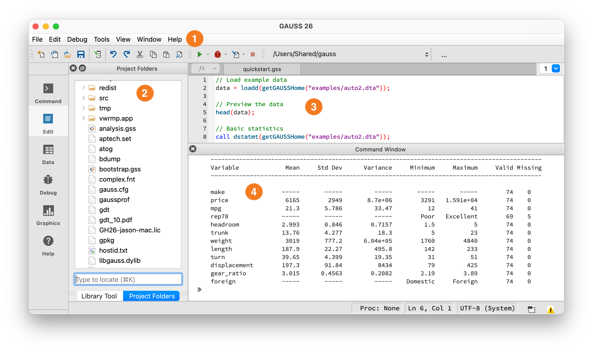
The GAUSS IDE workspace.#
① Toolbar — Shows your current working directory and the Run button (green arrow). Click it or press F5 to execute. ② Project Folders — File browser, similar to VS Code’s Explorer or Jupyter’s file browser. ③ Editor — Write programs here, similar to a VS Code editor tab or Jupyter code cell. ④ Command Window — Output appears here, similar to a terminal or Jupyter cell output. You can also type single lines at the >> prompt.
Debugging: Errors appear in the Output window with a line number – click it to jump to the error. Use the Variables panel (View > Variables) to inspect values at runtime. You can set breakpoints by clicking in the left margin of the editor, then step through code with the Debug menu. For quick debugging, insert print varname; statements.
Key Syntax Differences#
Feature |
Python/NumPy |
GAUSS |
|---|---|---|
Indexing |
0-based |
1-based |
Slicing end |
Exclusive |
Inclusive |
Assignment |
|
|
Matrix delimiter |
|
|
String quotes |
|
|
Statement end |
Newline |
Required |
All rows/cols |
|
|
String concat |
|
|
String equality |
|
|
Array/Matrix Creation#
# Python/NumPy
import numpy as np

A = np.array([[1, 2, 3],
              [4, 5, 6]])

zeros = np.zeros((3, 3))
ones = np.ones((3, 3))
identity = np.eye(3)
rand_uniform = np.random.rand(3, 3)
rand_normal = np.random.randn(3, 3)
// GAUSS
A = { 1 2 3,
      4 5 6 };

zeros_mat = zeros(3, 3);
ones_mat = ones(3, 3);
identity = eye(3);
rand_uniform = rndu(3, 3);
rand_normal = rndn(3, 3);
Sequences:
# Python/NumPy
np.arange(1, 6)           # [1, 2, 3, 4, 5]
np.arange(1, 3, 0.5)      # [1, 1.5, 2, 2.5]
np.linspace(0, 1, 5)      # 5 points from 0 to 1
// GAUSS
seqa(1, 1, 5);            // Column: start, increment, count
seqa(1, 0.5, 4);          // {1, 1.5, 2, 2.5}
seqa(0, 0.25, 5);         // {0, 0.25, 0.5, 0.75, 1}
Note: seqa takes (start, increment, count), not (start, stop). It always returns a column vector.
Operators#
Matrix vs element-wise is reversed!
# Python/NumPy
A * B             # Element-wise multiplication
A @ B             # Matrix multiplication
A ** 2            # Element-wise power
A / B             # Element-wise division
A.T               # Transpose
// GAUSS
A .* B;           // Element-wise multiplication (Python uses *)
A * B;            // Matrix multiplication (Python uses @)
A .^ 2;           // Element-wise power
A ./ B;           // Element-wise division
A';               // Transpose
Warning
Operators are reversed! Python’s * is element-wise; GAUSS’s * is matrix multiplication. Python’s @ is matrix multiply; GAUSS uses plain *. This will produce wrong results silently if you forget.
GAUSS has two forms of comparison operators. Without a dot, A > 0 returns a scalar – like Python’s np.all(A > 0). With a dot, A .> 0 returns an element-wise result – like Python’s A > 0:
# Python/NumPy
A > 0             # Element-wise comparison
A == B            # Element-wise equality
A != B            # Element-wise not-equal
A & B             # Element-wise AND (for arrays)
A | B             # Element-wise OR (for arrays)
// GAUSS
A .> 0;           // Element-wise comparison (like Python's A > 0)
A .== B;          // Element-wise equality
A .!= B;          // Element-wise not-equal
A .and B;         // Element-wise AND
A .or B;          // Element-wise OR
Warning
Two forms of comparison. A > 0 returns a scalar (1 if all elements satisfy the condition) – equivalent to Python’s np.all(A > 0). A .> 0 returns an element-wise array – equivalent to Python’s A > 0. Both forms exist for all comparison operators: >/.>, </.<, >=/.>=, <=/.<=, ==/.==, !=/.!=.
Warning
Python’s ``|`` is OR. GAUSS’s ``|`` is vertical concatenation. Writing condition1 | condition2 in GAUSS does NOT give you logical OR – it stacks the two vectors vertically. Use .or for element-wise OR and .and for element-wise AND. This will silently produce wrong results, not an error.
Concatenation#
# Python/NumPy
np.hstack([A, B])         # Horizontal
np.vstack([A, B])         # Vertical
"hello" + " world"        # String concatenation
// GAUSS
A ~ B;            // Horizontal concatenation (tilde)
A | B;            // Vertical concatenation (pipe)
a $+ b;           // String concatenation
For string arrays, use $~ (horizontal) and $| (vertical): "Domestic" $| "Foreign" creates a 2x1 string array.
String operators use the ``$`` prefix. In Python, == and + work on both strings and numbers. In GAUSS, string operations need a $ prefix: $+ (concatenation), $== (equality), $~ (horizontal join), $| (vertical join). Using == to compare strings will not work as expected.
Indexing#
This is the biggest difference. Python is 0-indexed; GAUSS is 1-indexed. Python slices are half-open [start:end); GAUSS slices are closed [start:end].
# Python/NumPy
A = np.array([[1, 2, 3],
              [4, 5, 6]])

A[0, 0]           # First element: 1
A[0, :]           # First row
A[:, 0]           # First column
A[0:2, :]         # Rows 0 and 1 (not 2!)
A[-1, :]          # Last row
// GAUSS
A = { 1 2 3,
      4 5 6 };

A[1, 1];          // First element: 1
A[1, .];          // First row (dot = all columns)
A[., 1];          // First column (dot = all rows)
A[1:2, .];        // Rows 1 and 2 (inclusive!)
A[rows(A), .];    // Last row (no negative indexing)
Key differences:
GAUSS uses
.for “all”, Python uses:or omits the indexGAUSS slices are inclusive:
A[1:3, .]gets rows 1, 2, and 3Python slices are half-open:
A[0:3, :]gets rows 0, 1, and 2No negative indexing in GAUSS. Use
rows(A)for last row,rows(A)-1for second-to-last.
Note
Most examples below use the auto2 dataset bundled with GAUSS. To run them, load it first:
auto2 = loadd(getGAUSSHome("examples/auto2.dta"));
Data Frames#
GAUSS dataframes are similar to pandas DataFrames – tabular data with named columns of different types.
Creating:
# Python/pandas
import pandas as pd
df = pd.DataFrame({
    "name": ["Alice", "Bob", "Charlie"],
    "age": [25, 30, 35],
    "score": [85.5, 92.0, 78.5]
})
// GAUSS
name = "Alice" $| "Bob" $| "Charlie";
age = { 25, 30, 35 };
score = { 85.5, 92.0, 78.5 };

// Build a dataframe by concatenating single-column dataframes
df = asDF(name, "name") ~ asDF(age, "age") ~ asDF(score, "score");
Loading data: GAUSS’s loadd() reads CSV, Excel, Stata, SAS, SPSS, and HDF5 files – see Data Import/Export below.
Viewing:
# Python/pandas
df.head()
df.shape
df.columns
df.dtypes
// GAUSS
head(df);                    // First 5 rows (same concept as pandas)
print rows(df) cols(df);    // Dimensions
print getcolnames(df)';     // Column names (column vector, transposed with ' for display)
getcoltypes(df);             // Column types (like df.dtypes)
Column and Row Selection#
# Python/pandas
df["price"]               # Column by name
df[["price", "mpg"]]      # Multiple columns
df.iloc[:, 2]             # Column by position
// GAUSS
df[., "price"];           // Column by name (dot = all rows)
df[., "price" "mpg"];     // Multiple columns (space-separated names)
df[., 3];                 // Column by position
# Python/pandas
df.iloc[0:5]                  # First 5 rows
df[df["age"] > 30]            # Filter by condition
df.iloc[[0, 2, 4]]           # Specific rows
// GAUSS
df[1:5, .];                          // First 5 rows
selif(df, df[., "age"] .> 30);       // Filter by condition (use selif, not brackets)
df[1|3|5, .];                        // Specific rows (| concatenates index values)
Warning
GAUSS does not support boolean indexing in brackets. In Python, df[condition] filters rows using a boolean array. In GAUSS, you must use selif(): selif(df, condition). Passing a boolean vector to brackets will not filter – it will try to use the 0s and 1s as row numbers.
Data Manipulation#
No method chaining – use intermediate variables. Python users chain operations with .method().method(). GAUSS has no chaining. Store intermediate results in variables:
# Python/pandas
result = (auto2
    .query("foreign == 0")
    .assign(price_k = lambda x: x["price"] / 1000)
    .sort_values("mpg")
    [["mpg", "price_k", "weight"]])
// GAUSS -- same workflow, intermediate variables
domestic = selif(auto2, auto2[., "foreign"] .== 0);
domestic = dfaddcol(domestic, "price_k", domestic[., "price"] ./ 1000);  // Add named column
domestic = sortc(domestic, "mpg");
result = domestic[., "mpg" "price_k" "weight"];
pandas method mapping:
Python (pandas) |
GAUSS |
|---|---|
|
|
|
|
|
|
|
|
|
|
|
|
|
|
Data Import/Export#
# Python/pandas
df = pd.read_csv("file.csv")
df = pd.read_stata("file.dta")
df = pd.read_excel("file.xlsx")
df.to_csv("output.csv")
// GAUSS - one function reads everything
data = loadd("file.csv");
data = loadd("file.dta");               // Stata
data = loadd("file.sas7bdat");           // SAS
data = loadd("file.xlsx");               // Excel

// Load specific variables with a formula string
data = loadd("auto2.dta", "mpg + rep78 + price");

// Load all variables except one
data = loadd("auto2.dta", ". -rep78");

// Export
saved(data, "output.csv");
saved(data, "output.xlsx");
Formula string quick reference: GAUSS uses formula strings in several contexts with different syntax:
Context |
Example |
Separator |
|---|---|---|
|
|
|
|
|
|
Bracket indexing |
|
Space separates names |
Type overrides |
|
Keywords wrap variable names |
Note
GAUSS formula strings are quoted strings ("y ~ x1 + x2"), not bare expressions like statsmodels’ ols("y ~ x1 + x2", data=df). The ~ separator works the same way in model formulas, but + in loadd() means “include this variable,” not “add to model.”
Missing Values#
Python uses np.nan (or None in pandas); GAUSS uses . (dot).
# Python/NumPy/pandas
np.isnan(x)               # Element-wise check
df.isna().any()           # Any missing?
df.dropna()               # Drop rows with any NaN
x[~np.isnan(x)]          # Keep non-missing
df.fillna(0)              # Replace NaN with 0
// GAUSS
x .== miss();             // Element-wise check (returns 1/0 vector)
ismiss(x);                // Any missing? (returns scalar 1 or 0)
packr(df);                // Drop rows with any missing value
selif(x, x .!= miss());  // Keep non-missing
missrv(x, 0);             // Replace missing with 0
Warning
ismiss is NOT element-wise. Python’s np.isnan(x) returns an array. GAUSS’s ismiss(x) returns a scalar (1 if any element is missing, 0 otherwise). For element-wise missing detection, use x .== miss().
Statistics#
# Python/NumPy
np.mean(x)
np.std(x, ddof=1)
np.sum(x)
np.min(x); np.max(x)
np.median(x)

# Column-wise on matrix
np.mean(X, axis=0)
np.sum(X, axis=0)
// GAUSS
meanc(x);     // Column mean (the 'c' suffix = column-wise)
stdc(x);      // Column std dev
sumc(x);      // Column sum
minc(x);      // Column min
maxc(x);      // Column max
median(x);    // Median

// Row-wise
meanr(X);     // Row mean (the 'r' suffix = row-wise)
sumr(X);      // Row sum
Descriptive statistics: Python’s df.describe() is dstatmt() in GAUSS:
call dstatmt(auto2[., "price" "mpg" "weight"]);
Warning
stdc uses N-1, not N. Python’s np.std(x) defaults to ddof=0 (population std dev). GAUSS’s stdc(x) always uses N-1 (sample std dev), equivalent to np.std(x, ddof=1). This will give different numbers if you forget.
Correlation:
# Python
np.corrcoef(x, y)        # 2x2 correlation matrix
np.corrcoef(X.T)         # Full correlation matrix
// GAUSS
corrx(x ~ y);             // 2x2 correlation matrix (~ is horizontal concat here)
corrx(X);                 // Full correlation matrix of all columns
Note
Like np.corrcoef, corrx() always returns a matrix. The difference is input format: np.corrcoef(x, y) takes two separate arrays, while corrx(x ~ y) takes a single concatenated matrix. To get a scalar correlation: corrx(x ~ y)[1, 2].
Linear Regression#
# Python/statsmodels
import statsmodels.api as sm
X = sm.add_constant(df[["mpg", "weight"]])
model = sm.OLS(df["price"], X).fit()
print(model.summary())

# Python/sklearn
from sklearn.linear_model import LinearRegression
model = LinearRegression().fit(X, y)
// GAUSS - print formatted summary (like model.summary())
call olsmt(auto2, "price ~ mpg + weight");
Tip
Use call olsmt(...) (with call) to print a formatted summary table to the screen without saving results to a variable. The call keyword discards return values.
Accessing results:
# Python/statsmodels
model.params              # Coefficients
model.bse                 # Standard errors
model.rsquared            # R-squared
model.resid               # Residuals
model.cov_params()        # Variance-covariance
// GAUSS
struct olsmtOut out;
out = olsmt(auto2, "price ~ mpg + weight");

print out.b;          // Coefficient estimates
print out.stderr;     // Standard errors
print out.rsq;        // R-squared
print out.resid;      // Residuals
print out.vc;         // Variance-covariance of estimates
Key olsmtOut members: b (coefficients), stderr (standard errors), vc (variance-covariance matrix), rsq (R-squared), resid (residuals), dwstat (Durbin-Watson), sigma (residual std dev), stb (standardized coefficients). See the olsmt() reference for the full list.
For robust or clustered standard errors, pass an olsmtControl structure – see the olsmt() reference for details.
Logistic regression (GLM):
# Python/statsmodels
import statsmodels.api as sm
model = sm.GLM(y, X, family=sm.families.Binomial()).fit()
// GAUSS
struct glmOut out;
out = glm(data, "admit ~ gre + gpa + rank", "binomial");
Quantile regression:
# Python/statsmodels
import statsmodels.formula.api as smf
mod = smf.quantreg("y ~ x1 + x2", df)
res = mod.fit(q=0.5)
// GAUSS (no package install needed)
struct qfitOut out;
out = quantileFit(data, "y ~ x1 + x2", 0.25 | 0.5 | 0.75);  // | builds a vector
Plotting#
Python users expect rich plotting from matplotlib/seaborn. GAUSS has a full graphics library:
# Python (matplotlib)
import matplotlib.pyplot as plt
plt.scatter(x, y)
plt.hist(x, bins=20)
plt.boxplot(data)

# Python (seaborn)
import seaborn as sns
sns.scatterplot(data=df, x="weight", y="mpg")
// GAUSS
plotXY(x, y);
plotScatter(x, y);
plotHist(x, 20);
plotBox(data, "value ~ group");
plotBar(labels, heights);
plotSurface(x, y, z);
Setting titles, labels, and legends uses a plotControl structure. Think of it as GAUSS’s equivalent of matplotlib’s plt.xlabel() / plt.title() calls, but configured before the plot call:
// Create a plot with title, labels, and legend
struct plotControl myPlot;
myPlot = plotGetDefaults("scatter");

plotSetTitle(&myPlot, "MPG vs Weight");
plotSetXLabel(&myPlot, "Weight (lbs)");
plotSetYLabel(&myPlot, "Miles per gallon");
plotSetLegend(&myPlot, "Domestic" $| "Foreign");

plotScatter(myPlot, auto2[., "weight"], auto2[., "mpg"]);
Subplots and saving:
# Python (matplotlib)
fig, axes = plt.subplots(2, 1)
plt.savefig("plot.png")
// GAUSS
plotLayout(2, 1, 1);            // 2 rows, 1 col, position 1
plotSave("plot.png", 640|480);  // Save with size (width|height in pixels)
Linear Algebra#
# Python/NumPy
np.linalg.inv(A)
np.linalg.det(A)
np.linalg.eig(A)
np.linalg.svd(A)
np.linalg.cholesky(A)
np.linalg.solve(A, b)
// GAUSS
inv(A);
invpd(A);             // Inverse (positive definite, faster)
det(A);
{ val, vec } = eigv(A);  // Eigenvalues and vectors (like np.linalg.eig)
eig(A);               // Eigenvalues only (like np.linalg.eigvals)
{ u, s, v } = svdcusv(A);
chol(A);              // Upper triangular (NumPy returns lower triangular)
b / A;                // Solve Ax = b (like np.linalg.solve(A, b))
Warning
``/`` is matrix division, not element-wise division. b / A solves the system Ax = b. Note the operand order is reversed from np.linalg.solve(A, b). For element-wise division, use ./. Python’s / is always element-wise on arrays; GAUSS’s / is not.
Optimization#
Python users doing custom optimization use scipy.optimize. GAUSS includes unconstrained and constrained optimization in the base package:
Python (scipy) |
GAUSS |
|---|---|
|
|
|
|
|
|
Key difference: Python passes functions as objects. GAUSS uses the & operator to pass a pointer to a named procedure. The & tells GAUSS to pass the procedure itself, not its result, so the optimizer can call it repeatedly with different parameter values:
# Python
from scipy.optimize import minimize

def my_obj(beta):
    resid = Y - X @ beta
    return resid @ resid

result = minimize(my_obj, x0)
// GAUSS -- named procedure; extra data passed as arguments
proc (1) = myObj(beta, Y, X);
    local resid;
    resid = Y - X * beta;
    retp(resid'resid);    // resid' * resid = sum of squared residuals
endp;

struct minimizeOut out;
out = minimize(&myObj, x0, Y, X);
For maximum likelihood estimation, the MLMT add-on provides maxlikmt() – a full MLE framework with standard errors, constraints, and convergence diagnostics.
In GAUSS, extra data arguments (Y and X above) are passed directly after the starting values and forwarded to your objective function automatically – no args= keyword needed.
Functions and Procedures#
# Python
def my_func(x, y):
    result = x + y
    return result
// GAUSS
proc (1) = my_func(x, y);
    local result;
    result = x + y;
    retp(result);
endp;
Key differences from Python:
proc (n) =declares the number of return valueslocaldeclares variables scoped to this procedure (required – see warning below)retp()returns valuesendpends the procedureNo default argument values. All arguments are positional.
No lambda functions. Use named procedures.
Multiple outputs:
# Python
def my_func(x):
    return x + 1, x - 1

a, b = my_func(5)
// GAUSS
proc (2) = my_func(x);
    local a, b;
    a = x + 1;
    b = x - 1;
    retp(a, b);
endp;

{ result_a, result_b } = my_func(5);
Warning
Variables are global by default. In Python, function variables are automatically local. In GAUSS, you must declare them with local inside proc or they become globals that persist after the procedure returns. Forgetting local creates hard-to-find bugs where procedures silently read or modify variables from the calling scope. This is a common beginner mistake – just make it a habit to declare local for every variable inside a proc.
Unlike Python, GAUSS procedures can be defined anywhere in your file – before or after the code that calls them. GAUSS compiles procedures in a separate pass.
Control Flow#
# Python
for i in range(1, 11):
    print(i)

if x > 0:
    print("positive")
elif x < 0:
    print("negative")
else:
    print("zero")

while x > 0:
    x -= 1
// GAUSS
for i (1, 10, 1);
    print i;
endfor;

if x > 0;
    print "positive";
elseif x < 0;
    print "negative";
else;
    print "zero";
endif;

do while x > 0;
    x = x - 1;
endo;
Note: GAUSS requires semicolons after control statements (if, for, else, etc.). Inside a proc, remember to declare loop variables with local (see the warning above) or they become globals.
Common Function Translations#
Description |
Python/NumPy |
GAUSS |
|---|---|---|
Natural log |
|
|
Log base 10 |
|
|
Column mean |
|
|
Row mean |
|
|
Column sum |
|
|
Cumulative sum |
|
|
Sort by column |
|
|
Find indices |
|
|
Filter rows |
|
|
Remove missing rows |
|
|
Replace missing |
|
|
Check NaN (any) |
|
|
Check NaN (element) |
|
|
Flip rows |
|
|
Create diagonal matrix |
|
|
Reshape |
|
|
Flatten to column |
|
|
Full SVD |
|
|
Number to string |
|
|
Formatted output |
|
|
Random uniform |
|
|
Random normal |
|
|
Set seed |
|
|
|
|
|
Comment |
|
|
Warning
log vs ln: In Python, np.log is the natural logarithm. In GAUSS, log is base 10 and ln is natural. This will silently give wrong results if you don’t catch it.
Python Package to GAUSS Mapping#
Python assembles workflows from packages. GAUSS includes most of this in the base installation:
Python Package |
GAUSS Equivalent |
|---|---|
|
Base GAUSS ( |
|
Base GAUSS ( |
|
Base GAUSS ( |
|
Base GAUSS ( |
|
Base GAUSS ( |
|
Base GAUSS ( |
|
TSMT add-on |
|
TSMT add-on |
Time series users: If your work involves ARIMA, VAR, GARCH, impulse response functions, or forecasting, you will use the TSMT add-on. Key functions: arimaFit(), svarFit() (structural VAR), varmaFit(), varmaPredict(). See the time series blog for complete worked examples.
Common Gotchas#
Indexing starts at 1. The first element is
A[1, 1], notA[0, 0].Slices are inclusive.
A[1:3, .]includes rows 1, 2, AND 3. Python’sA[0:3]excludes index 3.Operators are reversed.
*is matrix multiply,.*is element-wise (opposite of NumPy!).Semicolons required. Every statement ends with
;.Dot not colon for “all”. “All rows” is
df[., 1]notdf[:, 0]. But:works for ranges:df[1:5, .].String quotes. Only double quotes
"string"work.No negative indexing. Use
rows(A)andcols(A)instead.The ``call`` keyword. Use
call functionName(...)to run a function and discard its return value. This is the GAUSS equivalent of running a function for its side effects (like printing).String operators need ``$``.
==won’t compare strings. Use$==for string equality,$+for concatenation.
For operator gotchas (* vs .*, | vs .or, dotted comparisons, / vs ./, log vs ln), variable scoping (local), and boolean indexing (selif), see the inline warnings throughout this guide.
Putting It Together#
Here is a complete, runnable example that loads data, filters it, plots it, runs a regression, and prints the results. Running this prints the OLS summary to the Output window and opens a scatter plot.
// Load the auto2 dataset bundled with GAUSS
auto2 = loadd(getGAUSSHome("examples/auto2.dta"));

// Keep only domestic cars (foreign == 0)
domestic = selif(auto2, auto2[., "foreign"] .== 0);

// Quick scatter plot with title and labels
struct plotControl myPlot;
myPlot = plotGetDefaults("scatter");
plotSetTitle(&myPlot, "Weight vs MPG (Domestic Cars)");
plotSetXLabel(&myPlot, "Weight (lbs)");
plotSetYLabel(&myPlot, "Miles per gallon");
plotScatter(myPlot, domestic[., "weight"], domestic[., "mpg"]);

// Run OLS: how does weight affect fuel efficiency?
struct olsmtOut out;
out = olsmt(domestic, "mpg ~ weight");

// Print key results
print out.b;         // Coefficient estimates
print out.stderr;    // Standard errors
print out.rsq;       // R-squared
What’s Next?#
GAUSS Quickstart – 10-minute introduction to GAUSS basics
Running Existing Code – If you inherited GAUSS code and need to get it running
Data Management – Loading, cleaning, and reshaping data
Textbook Examples – Worked examples from Greene (Econometric Analysis) and Brooks (Introductory Econometrics for Finance)
Command Reference – Browse all 1,000+ built-in functions
Econometrics blog – Fully worked examples covering regression, panel data, hypothesis testing, and more
Time series blog – ARIMA, VAR, GARCH, cointegration, and forecasting tutorials with complete code
See also
loadd(), olsmt(), glm(), quantileFit(), minimize(), plotXY(), packr(), selif()