Introduction to GAUSS for MATLAB Users#
If you work with matrices, optimization, and numerical computing in MATLAB, you’ll find GAUSS handles these the same way – with differences in syntax and a stronger focus on econometrics and statistics. This guide maps MATLAB concepts, syntax, and workflows to their GAUSS equivalents.
Note
This guide is written for GAUSS 26. Some features (such as repmat(), findIdx(), diagmat(), and the colon operator for sequences) require GAUSS 26.0.1 or later.
Where to type code:
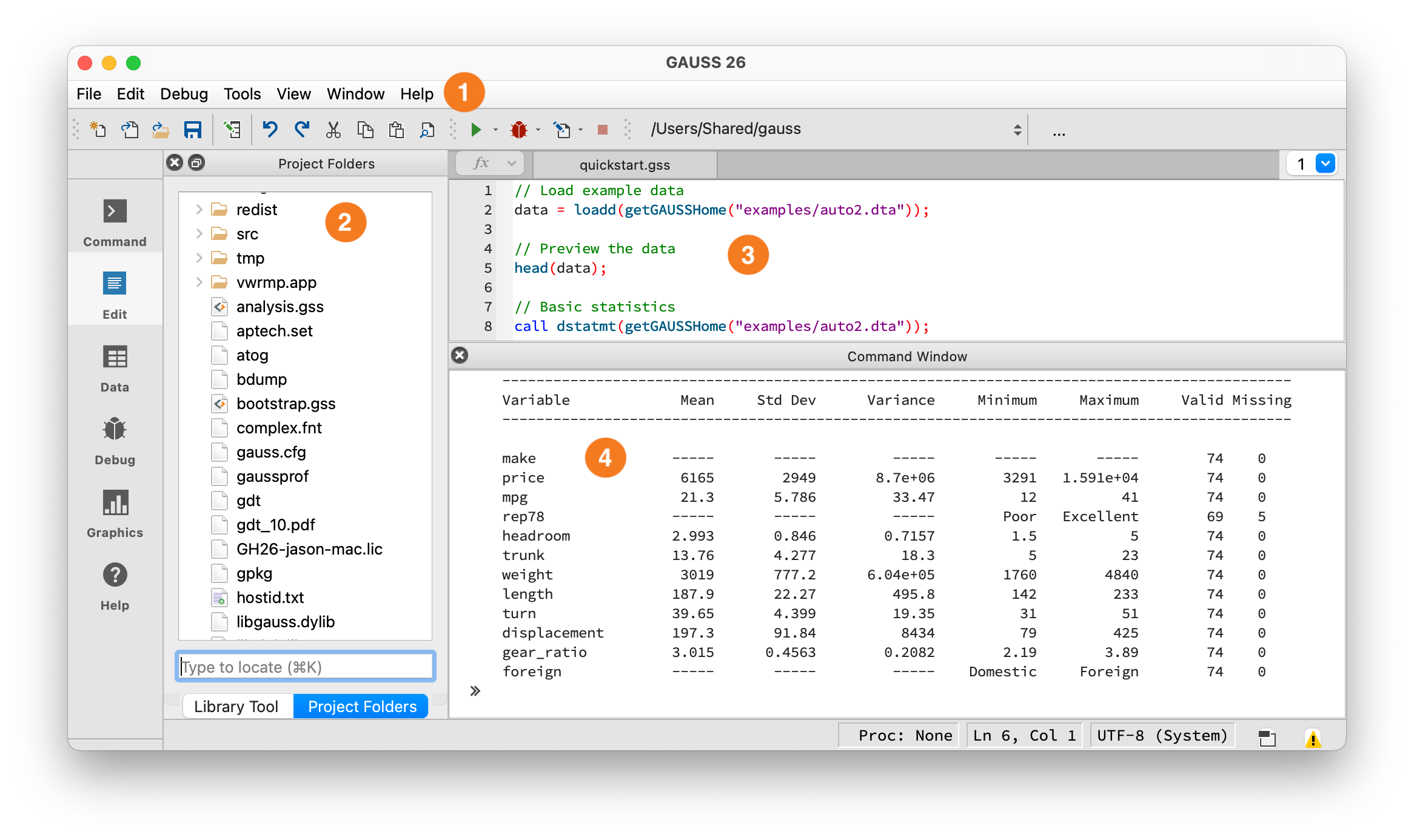
The GAUSS IDE workspace.#
① Toolbar — Shows your current working directory and the Run button (green arrow). Click it or press F5 to execute. ② Project Folders — File browser, similar to MATLAB’s Current Folder. ③ Editor — Write programs here, similar to the MATLAB Editor. ④ Command Window — Output appears here, similar to MATLAB’s Command Window. You can also type single lines at the >> prompt.
Debugging: Errors appear in the Output window with a line number – click it to jump to the error. Use the Variables panel (View > Variables) to inspect values at runtime. You can set breakpoints by clicking in the left margin of the editor, then step through code with the Debug menu. For quick debugging, insert print varname; statements.
Inspecting structures: To see what fields an output structure contains, use print – for example, print out; displays all members and their values. To see just the field names, check the structure definition in the Command Reference (press F1 on the function name).
How GAUSS Differs from MATLAB#
GAUSS shares MATLAB’s matrix-first philosophy but is oriented around statistics and econometrics rather than engineering. Here are the practical differences that affect your daily coding:
Dataframes are matrices: Named columns and typed variables, but you can do matrix algebra on them directly – no
table2arrayconversion step.Column-wise by default: Statistical functions operate on columns (
meanc,stdc,sumc), matching the convention that columns are variables and rows are observations.Formula strings for estimation: Model specification uses
"y ~ x1 + x2"syntax (similar to R). Categorical variables are handled automatically.Structures for output: Estimation results are returned in structures with named members (
out.b,out.stderr), similar to MATLAB structs.No toolbox fees: OLS, GLM, quantile regression, optimization, and plotting are all included in the base package – no extra toolboxes required.
Key Syntax Differences#
Feature |
MATLAB |
GAUSS |
|---|---|---|
Indexing |
1-based |
1-based (same) |
Matrix delimiter |
|
|
Row separator |
|
|
String quotes |
|
|
Statement end |
Optional |
Required |
All rows/cols |
|
|
Concatenate horiz |
|
|
Concatenate vert |
|
|
Solve |
|
|
Note
Most examples below use the auto2 dataset bundled with GAUSS. To run them, load it first:
auto2 = loadd(getGAUSSHome("examples/auto2.dta"));
Matrix Creation#
% MATLAB
A = [1 2 3; 4 5 6; 7 8 9]
// GAUSS
A = { 1 2 3, 4 5 6, 7 8 9 };
Note: GAUSS uses braces { } and commas between rows. Semicolons end statements, not rows. Unlike MATLAB, newlines are not row separators – you must use commas.
Special matrices:
% MATLAB
zeros(3,3)
ones(3,3)
eye(3)
rand(3,3)
randn(3,3)
// GAUSS
zeros(3, 3);
ones(3, 3);
eye(3);
rndu(3, 3);    // Uniform [0,1]
rndn(3, 3);    // Standard normal
Sequences:
% MATLAB
1:5           % Row vector [1 2 3 4 5]
1:0.5:3       % [1 1.5 2 2.5 3]
linspace(0,1,5)
// GAUSS
1:5;                 // Column vector {1, 2, 3, 4, 5} (NOTE: MATLAB gives a row vector)
1:0.5:3;             // Column vector {1, 1.5, 2, 2.5, 3}
seqa(1, 1, 5);       // Column vector, start=1, inc=1, n=5
seqa(0, 0.25, 5);    // Column vector {0, 0.25, 0.5, 0.75, 1}
Note: MATLAB’s colon operator produces row vectors; GAUSS produces column vectors. MATLAB’s linspace(0, 1, 5) takes start, end, and count. GAUSS’s seqa() takes start, increment, and count – you must compute the step size yourself: seqa(0, (1-0)/(5-1), 5).
Indexing#
Both languages use 1-based indexing, but the “all elements” syntax differs:
% MATLAB
A(1,1)        % Element
A(1,:)        % First row
A(:,1)        % First column
A(1:2,:)      % Rows 1-2
A(end,:)      % Last row
A(end-2:end,:)  % Last 3 rows
// GAUSS
A[1, 1];          // Element
A[1, .];          // First row (dot = all)
A[., 1];          // First column
A[1:2, .];        // Rows 1-2
A[rows(A), .];    // Last row (no 'end' keyword)
A[rows(A)-2:rows(A), .];  // Last 3 rows
GAUSS dataframes also support indexing by column name:
auto2[., "mpg"];              // One column by name
auto2[., "mpg" "weight"];    // Multiple columns (space-separated)
auto2[1:10, "mpg"];          // First 10 rows of mpg
Key difference: MATLAB uses : for “all”, GAUSS uses .. Use rows(A) and cols(A) where MATLAB uses end.
Operators#
Element-wise vs. matrix operations:
% MATLAB
A * B         % Matrix multiplication
A .* B        % Element-wise multiplication
A .^ 2        % Element-wise power
A'            % Transpose
// GAUSS
A * B;        // Matrix multiplication (same)
A .* B;       // Element-wise multiplication (same)
A .^ 2;       // Element-wise power (same)
A';           // Transpose (same)
Element-wise arithmetic operators (.* ./ .^) and transpose (') work the same in both languages.
Comparison operators are different. GAUSS uses dot-prefixed operators for element-wise comparison:
% MATLAB
A > 0         % Element-wise comparison
A == B        % Element-wise equality
A ~= B        % Element-wise not-equal
A & B         % Element-wise AND
A | B         % Element-wise OR (also vertical concat in GAUSS!)
// GAUSS
A .> 0;       // Element-wise comparison (dot prefix required)
A .== B;      // Element-wise equality
A .!= B;      // Element-wise not-equal (.ne also works)
A .and B;     // Element-wise AND
A .or B;      // Element-wise OR
Warning
Comparison operators need dots. In MATLAB, A > 0 is element-wise. In GAUSS, A > 0 without the dot tests whether all elements satisfy the condition (returns a scalar). Use .> for element-wise results. This is the most common source of bugs for MATLAB migrants.
Concatenation#
% MATLAB
[A B]         % Horizontal concatenation
[A; B]        % Vertical concatenation
// GAUSS
A ~ B;        // Horizontal concatenation (tilde)
A | B;        // Vertical concatenation (pipe)
For strings, use $~ (horizontal) and $| (vertical): "Domestic" $| "Foreign" creates a 2x1 string array.
Example:
A = { 1 2, 3 4 };
B = { 5, 6 };

print A ~ B;   // [1 2 5; 3 4 6]
print A | B';  // [1 2; 3 4; 5 6]
Filtering and Selection#
MATLAB uses logical indexing directly. GAUSS uses selif() with element-wise comparison operators:
% MATLAB
A(A(:,1) > 5, :)              % Rows where column 1 > 5
data(data.price > 10000, :)   % Filter table by condition
// GAUSS
selif(A, A[., 1] .> 5);                      // Rows where column 1 > 5
selif(auto2, auto2[., "price"] .> 10000);    // Filter by condition

// Combine conditions
mask = auto2[., "mpg"] .> 20 .and auto2[., "price"] .< 8000;
cheap_efficient = selif(auto2, mask);
Note the .> operator: GAUSS requires the dot prefix for element-wise comparison (see Operators above).
Missing values: MATLAB uses NaN and isnan; GAUSS uses . (dot) and provides several tools:
% MATLAB
clean = rmmissing(data);           % Drop rows with any NaN
data(isnan(data)) = 0;             % Replace NaN with 0
mask = ~isnan(data(:,3));          % Rows where column 3 is not NaN
// GAUSS
clean = packr(data);               // Drop rows with any missing value
data = missrv(data, 0);            // Replace missings with 0
mask = data[., 3] .!= miss(1, 1); // Rows where column 3 is not missing
packr() is the workhorse – it removes any row containing a missing value. Use missrv() to replace missings with a specific value. For element-wise missing detection, use x .== miss(1, 1) (see the Common Function Translations table).
Data Import/Export#
% MATLAB
data = readtable('file.csv');
data = xlsread('file.xlsx');
writetable(data, 'output.csv')
// GAUSS - loadd reads CSV, Excel, Stata, SAS, SPSS, HDF5
data = loadd("file.csv");
data = loadd("file.xlsx");
data = loadd("auto2.dta");           // Stata
data = loadd("survey.sas7bdat");     // SAS

// Load specific variables with a formula string
data = loadd("auto2.dta", "mpg + rep78 + price");

// Load all variables except one
data = loadd("auto2.dta", ". -rep78");

// Export
saved(data, "output.csv");
saved(data, "output.xlsx");
saved(data, "output.gdat");          // GAUSS format
getGAUSSHome() returns the path to GAUSS’s installation directory. Use it to access bundled example datasets: loadd(getGAUSSHome("examples/auto2.dta")).
Formula string quick reference: GAUSS uses formula strings in several contexts with slightly different syntax:
Statistics and Econometrics#
Unlike MATLAB, where fitlm, fitglm, and optimization functions require the Statistics or Optimization Toolbox, GAUSS includes all of these in the base package.
Basic statistics:
% MATLAB
mean(x)       % Column means
std(x)        % Column std devs
sum(x)        % Column sums
cov(x)        % Covariance matrix
// GAUSS
meanc(x);     // Column means (the 'c' suffix = column-wise)
stdc(x);      // Column std devs
sumc(x);      // Column sums
vcx(x);       // Covariance matrix
OLS regression:
% MATLAB (Statistics Toolbox)
mdl = fitlm(X, y);
mdl.Coefficients
mdl.Residuals.Raw
// GAUSS
struct olsmtOut out;
out = olsmt(auto2, "price ~ mpg + weight");

// Access results through the output structure
print out.b;          // Coefficient estimates
print out.stderr;     // Standard errors
print out.rsq;        // R-squared
Key olsmtOut members: b (coefficients), stderr (standard errors), vc (variance-covariance matrix), rsq (R-squared), resid (residuals), dwstat (Durbin-Watson), sigma (residual std dev), stb (standardized coefficients). To compute t-statistics and p-values: t = out.b ./ out.stderr. See the olsmt() reference for the full list.
Tip
Use call olsmt(...) (with call) to print a formatted summary table to the screen without saving results to a variable. The call keyword discards return values.
Logistic regression (GLM):
% MATLAB (Statistics Toolbox)
mdl = fitglm(X, y, 'Distribution', 'binomial');
// GAUSS
struct glmOut out;
out = glm(data, "admit ~ gre + gpa + rank", "binomial");
Quantile regression:
// GAUSS (no MATLAB built-in equivalent)
struct qfitOut out;
out = quantileFit(data, "y ~ x1 + x2", 0.25 | 0.5 | 0.75);
For robust or clustered standard errors, pass an olsmtControl structure – see the olsmt() reference for details.
Plotting#
MATLAB users expect rich plotting. GAUSS has a full graphics library:
% MATLAB
plot(x, y)
scatter(x, y)
histogram(x, 20)
bar(labels, heights)
surf(X, Y, Z)
subplot(2, 1, 1)
title('My Plot')
xlabel('X axis')
saveas(fig, 'plot.png')
// GAUSS
plotXY(x, y);
plotScatter(x, y);
plotHist(x, 20);
plotBar(labels, heights);
plotSurface(x, y, z);
plotLayout(2, 1, 1);
// Title and labels use a plotControl structure (see below)
plotSave("plot.png");
Setting titles, labels, and legends uses a plotControl structure:
// Create a plot with title, labels, and legend
struct plotControl myPlot;
myPlot = plotGetDefaults("xy");

plotSetTitle(&myPlot, "MPG vs Weight");
plotSetXLabel(&myPlot, "Weight (lbs)");
plotSetYLabel(&myPlot, "Miles per gallon");
plotSetLegend(&myPlot, "Domestic" $| "Foreign");

plotXY(myPlot, auto2[., "weight"], auto2[., "mpg"]);
Quick plotting example:
// Sine wave -- no plotControl needed for simple plots
x = seqa(0, 0.1, 63);   // 0 to ~2*pi
plotXY(x, sin(x));
Optimization#
GAUSS includes unconstrained and constrained optimization in the base package.
Key difference: MATLAB uses anonymous functions (@(x) ...) to pass objectives. GAUSS uses the & operator to pass a pointer to a named procedure. Extra data arguments are passed after the starting values:
% MATLAB -- anonymous function captures Y, X via closure
f = @(beta) sum((Y - X*beta).^2);
result = fminunc(f, x0);
// GAUSS -- named procedure; extra data passed as arguments
proc (1) = myObj(beta, Y, X);
    local resid;
    resid = Y - X * beta;
    retp(resid'resid);    // resid' * resid = sum of squared residuals
endp;

struct minimizeOut out;
out = minimize(&myObj, x0, Y, X);
For constrained optimization with linear or nonlinear constraints, see sqpSolve(). For systems of nonlinear equations, see eqSolve().
Linear Algebra#
% MATLAB
inv(A)
det(A)
eig(A)
[V,D] = eig(A)
svd(A)
chol(A)
rank(A)
A \ b          % Solve Ax = b
// GAUSS
inv(A);
invpd(A);             // Inverse (positive definite, faster)
det(A);
eig(A);               // Returns eigenvalues only
{ val, vec } = eigv(A);  // Eigenvalues and vectors
{ u, s, v } = svdcusv(A);
chol(A);
rank(A);
b / A;                // Solve Ax = b
Solving linear systems: GAUSS uses the / operator: b / A solves Ax = b. Use solpd() for positive definite systems or olsqr() for QR-based least squares.
Warning
eigv return order is reversed. MATLAB’s [V, D] = eig(A) returns eigenvectors first, then eigenvalues. GAUSS’s { val, vec } = eigv(A) returns eigenvalues first, then eigenvectors. Swapping these produces wrong results silently.
Functions and Procedures#
% MATLAB
function y = square(x)
    y = x.^2;
end
// GAUSS
proc (1) = square(x);
    local y;        // Must declare local variables (see Gotcha #8)
    y = x.^2;
    retp(y);
endp;
Key differences:
GAUSS uses
proc/endpinstead offunction/endReturn values use
retp()not assignmentNumber of outputs declared in
proc (n) =
Multiple outputs:
% MATLAB
function [a, b] = myFunc(x)
    a = x + 1;
    b = x - 1;
end
// GAUSS
proc (2) = myFunc(x);
    local a, b;
    a = x + 1;
    b = x - 1;
    retp(a, b);
endp;

// Call it
{ result1, result2 } = myFunc(5);
Control Flow#
Loops and conditionals are similar:
% MATLAB
for i = 1:10
    disp(i)
end

if x > 0
    disp('positive')
elseif x < 0
    disp('negative')
else
    disp('zero')
end
// GAUSS
for i (1, 10, 1);
    print i;
endfor;

if x > 0;
    print "positive";
elseif x < 0;
    print "negative";
else;
    print "zero";
endif;
While loops:
% MATLAB
while x > 0
    x = x - 1;
end
// GAUSS
do while x > 0;
    x = x - 1;
endo;
Note: GAUSS requires semicolons after control statements (if, for, else, etc.). Inside a proc, remember to declare loop variables with local (see Gotcha #9) or they become globals: local i; for i (1, 10, 1); ... endfor;
Common Function Translations#
Functions with different names:
Functions with the same name: repmat, unique, abs, exp, ceil, floor, round, rank, inv, det, chol, eye, zeros, ones, fft
Warning
reshape fill order differs. MATLAB’s reshape fills column-major (down columns first). GAUSS’s reshape fills row-major (across rows first). The same input will produce different matrix layouts – silently, with no error.
Note
diag vs diagmat: MATLAB’s diag both creates and extracts diagonal matrices. In GAUSS, diag(A) only extracts the diagonal. To create a diagonal matrix from a vector, use diagmat(v).
Warning
log vs ln: In MATLAB, log is the natural logarithm. In GAUSS, log is base 10 and ln is natural. This will silently give wrong results if you don’t catch it.
Toolbox-to-Package Mapping#
MATLAB functionality is split across paid toolboxes. GAUSS includes most of it in the base package:
MATLAB Toolbox |
GAUSS Equivalent |
|---|---|
Statistics & Machine Learning |
Base GAUSS (OLS, GLM, quantile reg, etc.) |
Optimization Toolbox |
Base GAUSS ( |
Econometrics Toolbox |
Base GAUSS + TSMT (time series add-on) |
Signal Processing Toolbox |
|
Financial Toolbox |
Fanpac (add-on) |
Time series users: If your work involves ARIMA, VAR, GARCH, impulse response functions, or forecasting, you will use the TSMT add-on. Key functions: arimaFit(), svarFit() (structural VAR), varmaFit(), varmaPredict(). For maximum likelihood estimation, see maxlikmt(). See the time series blog for complete worked examples.
Common Gotchas#
Semicolons are required. Every statement must end with
;Braces not brackets. Matrices use
{ }not[ ]Dot not colon for “all”. “All rows” is
A[.,1]notA(:,1). But:works for ranges:A[1:5, .].Comparison operators need dots. Element-wise comparison uses
.>,.<,.==,.!=. Without the dot,>tests if all elements satisfy the condition. This is the most common bug for MATLAB migrants.Slash not backslash. Use
b/Ainstead ofA\blog means base 10. MATLAB
log= natural log. GAUSSlog= base 10. Uselnfor natural log.String quotes. Only double quotes
"string"workProcedure syntax. Use
proc/endp/retpnotfunction/end/returnLocal variables are not automatic. In MATLAB, function variables are local by default. In GAUSS, you must declare them with
localinsideprocor they become global. Forgettinglocalcreates hard-to-find bugs where procedures silently read or modify variables from the calling scope.No ``end`` keyword for indexing. Use
rows(A)instead ofend. For the last 5 rows:A[rows(A)-4:rows(A), .]The ``call`` keyword. Use
call functionName(...)to run a function and discard its return value. This is common for estimation functions:call olsmt(data, "y ~ x")prints the summary table without saving results.
Putting It Together#
Here is a complete, runnable example that loads data, filters it, plots it, runs a regression, and prints the results:
// Load the auto2 dataset bundled with GAUSS
auto2 = loadd(getGAUSSHome("examples/auto2.dta"));

// Keep only domestic cars (foreign == 0)
domestic = selif(auto2, auto2[., "foreign"] .== 0);

// Quick scatter plot
plotScatter(domestic[., "weight"], domestic[., "mpg"]);

// Run OLS: how does weight affect fuel efficiency?
struct olsmtOut out;
out = olsmt(domestic, "mpg ~ weight");

print out.b;         // Coefficient estimates
print out.stderr;    // Standard errors
print out.rsq;       // R-squared
What’s Next?#
GAUSS Quickstart – 10-minute introduction to GAUSS basics
Running Existing Code – If you inherited GAUSS code and need to get it running
Data Management – Loading, cleaning, and reshaping data
Textbook Examples – Worked examples from Greene (Econometric Analysis) and Brooks (Introductory Econometrics for Finance)
Command Reference – Browse all 1,000+ built-in functions
Graphics documentation – Plotting functions, customization, and export
saved()– Export data to CSV, Excel, or other formatsUser Guide – Installing and managing add-on modules
Econometrics blog – Fully worked examples covering regression, panel data, hypothesis testing, and more
Time series blog – ARIMA, VAR, GARCH, cointegration, and forecasting tutorials with complete code
Programming blog – Loops, string handling, data manipulation, and general GAUSS programming
See also
loadd(), olsmt(), glm(), quantileFit(), minimize(), plotXY(), fft()