Chapter 5: Estimation and Hypothesis Testing of the CAPM#
Example 1: Estimate the CAPM Regression Equation#
This example demonstrates how to estimate the model:
Getting Started#
To run this example on your own you will need to install the BrooksEconFinLib package. This package houses all examples and associated data.
How to#
Step One: Load the data#
To start, load the relevant variables from the dataset using loadd() and a formula string.
To replicate this example, we will load the following variables:
Date - Observation date.
SandP - S&P 500 index.
USTB3M - Three month T-bill yields. (Note that our data has already been converted to monthly).
FORD - Stock prices.
GE - Stock prices.
MICROSOFT - Stock prices.
ORACLE - Stock prices.
// Create file name with full path
data_file = getGAUSSHome() $+ "pkgs/BrooksEcoFinLib/examples/capm.csv";

// Load all variables from the CSV file
data_org = loadd(data_file, "date(Date) + FORD + SandP + USTB3M");

// Print the first 5 rows
head(data_org);
      Date             FORD            SandP           USTB3M
2002-01-01        15.300000        1130.2000       0.14000000
2002-02-01        14.880000        1106.7300       0.14666667
2002-03-01        16.490000        1147.3900       0.15250000
2002-04-01        16.000000        1076.9200       0.14583333
2002-05-01        17.650000        1067.1400       0.14666667
Further reading: Data management guide
Function reference: getGAUSSHome(), head(), loadd()
Step Two: Transform data#
Our data transformation starts by defining a procedure to compute log returns and using that procedure to compute log returns of the SandP and FORD variables.
Previous versions of our lnDiff procedure removed the missing observation from the first element of the return value. This time we want to keep the missing observation, because it is more convenient to assign the entire column than a partial column.
We could just remove the call to packr() from the version of lnDiff in our previous example. However, we will use this chance to show you how to use optional inputs to GAUSS procedures.
/*
**  Procedure to compute log differences
**
** The second input, '...', tells GAUSS
** that this procedure can accept extra
** optional inputs
*/
proc (1) = lnDiff(x, ...);
    local x_diff, trim1;

    // If an optional input is passed in,
    // set 'trim1' equal to its value,
    // otherwise set trim equal to 1.
    trim1 = dynargsGet(1, 1);

    x_diff =  100 * ln(x ./ lagn(x, 1));

    // If 'trim1' is not equal to 0.
    if trim1;
        // Trim 1 row from the top
        // and 0 from the bottom
        x_diff = trimr(x_diff, 1, 0);
    endif;

    retp(x_diff);
endp;

// Create a new dataframe with the continuously
// compounded returns of 'FORD' and 'SandP'
trim_1 = 0;
returns = lnDiff(data_org[., "FORD" "SandP"], trim_1);

// Set the variable names
returns = asDF(returns, "ret_ford", "ret_sandp");

head(returns);
  ret_ford        ret_sandp
         .                .
-2.7834799       -2.0984861
 10.273611        3.6080107
-3.0165414       -6.3384655
 9.8147061      -0.91229691
We will finish our data preparation by computing the excess return of SandP and FORD and then combining all the variables into one dataframe named, data.
// Create a datframe with the excess return of 'SandP' and 'FORD', by
// subtracting 'USTB3M' from both return variables computed above
er = returns - data_org[.,"USTB3M"];

// The excess return variables will be in the same order
// as the return variables in 'returns'. So make sure the
// variable names are in the right order.
er = asDF(er, "erford", "ersandp");

// Add the 'Date' and 'USTB3M' variables to the front
// of 'data using the horizontal concatenation operator '~'.
data = data_org[.,"Date" "USTB3M"] ~ er ~ returns;

head(data);
      Date         ret_ford        ret_sandp           USTB3M           erford          ersandp
2002-01-01                .                .       0.14000000                .                .
2002-02-01       -2.7834799       -2.0984861       0.14666667       -2.9301466       -2.2451528
2002-03-01        10.273611        3.6080107       0.15250000        10.121111        3.4555107
2002-04-01       -3.0165414       -6.3384655       0.14583333       -3.1623748       -6.4842988
2002-05-01        9.8147061      -0.91229691       0.14666667        9.6680394       -1.0589636
Further reading:
Function reference: asdf(), dynargsGet(), loadd(), ln(), trimr()
Step Three: Plot data#
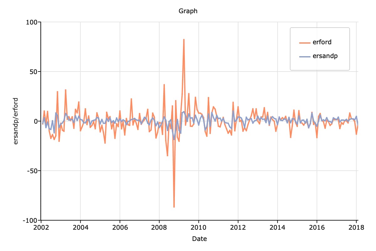
We can create the above time series plot with the following code:
// Set size of graph
plotCanvasSize("px", 600 | 400);

// Declare plotControl structure
// and fill with default settings
struct plotControl plt;
plt = plotGetDefaults("xy");

plotSetYLabel(&plt, "ersandp/erford");
plotSetTitle(&plt, "Graph");
plotSetGrid(&plt, "on");

// Draw the plot using a formula string
plotXY(data, "ersandp + erford ~ Date");
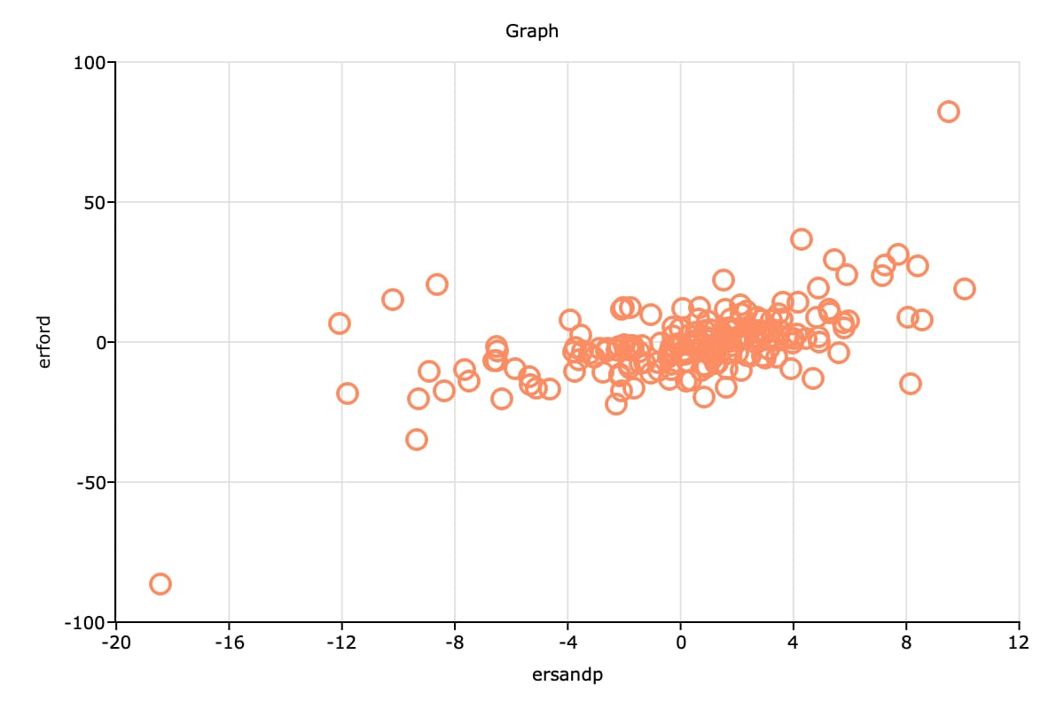
The code below will create the above scatter plot.
// Open a new graph window so we don't
// overwrite the graph we just created
plotOpenWindow();

// Fill 'plt' with default settings for scatter plots
struct plotControl plt;
plt = plotGetDefaults("scatter");

plotSetTitle(&plt, "Graph");
plotSetGrid(&plt, "on");

// Plot 'erford' vs 'ersandp' using a formula string
plotScatter(plt, data, "erford ~ ersandp");
Further reading: Basic GAUSS Graph Customization
Function reference: plotcanvassize(), plotgetdefaults(), plotOpenWindow(), plotScatter(), plotSetGrid(), plotSetTitle(), plotSetYLabel()
Step Four: Compute regression#
// Compute the regression:
//     'erford = a + B*ersandp + err
// and print results
call olsmt(data, "erford ~ ersandp");
Valid cases:                   193      Dependent variable:              erford
Missing cases:                   1      Deletion method:               Listwise
Total SS:                34741.345      Degrees of freedom:                 191
R-squared:                   0.337      Rbar-squared:                     0.334
Residual SS:             23019.606      Std error of est:                10.978
F(1,191):                   97.258      Probability of F:                 0.000

                         Standard                 Prob   Standardized  Cor with
Variable     Estimate      Error      t-value     >|t|     Estimate    Dep Var
-------------------------------------------------------------------------------

CONSTANT    -0.955984    0.793085     -1.2054     0.230       ---         ---
ersandp       1.88976     0.19162     9.86197     0.000    0.580862    0.580862
Function reference: olsmt()