Introduction to GAUSS for Stata Users#
A practical guide to doing common Stata operations in GAUSS, with references for deeper exploration.
GAUSS auto-detects variable types, previews your data, and generates reusable code. Watch the video to see a full workflow from data import through ARIMA estimation.#
The GAUSS IDE#
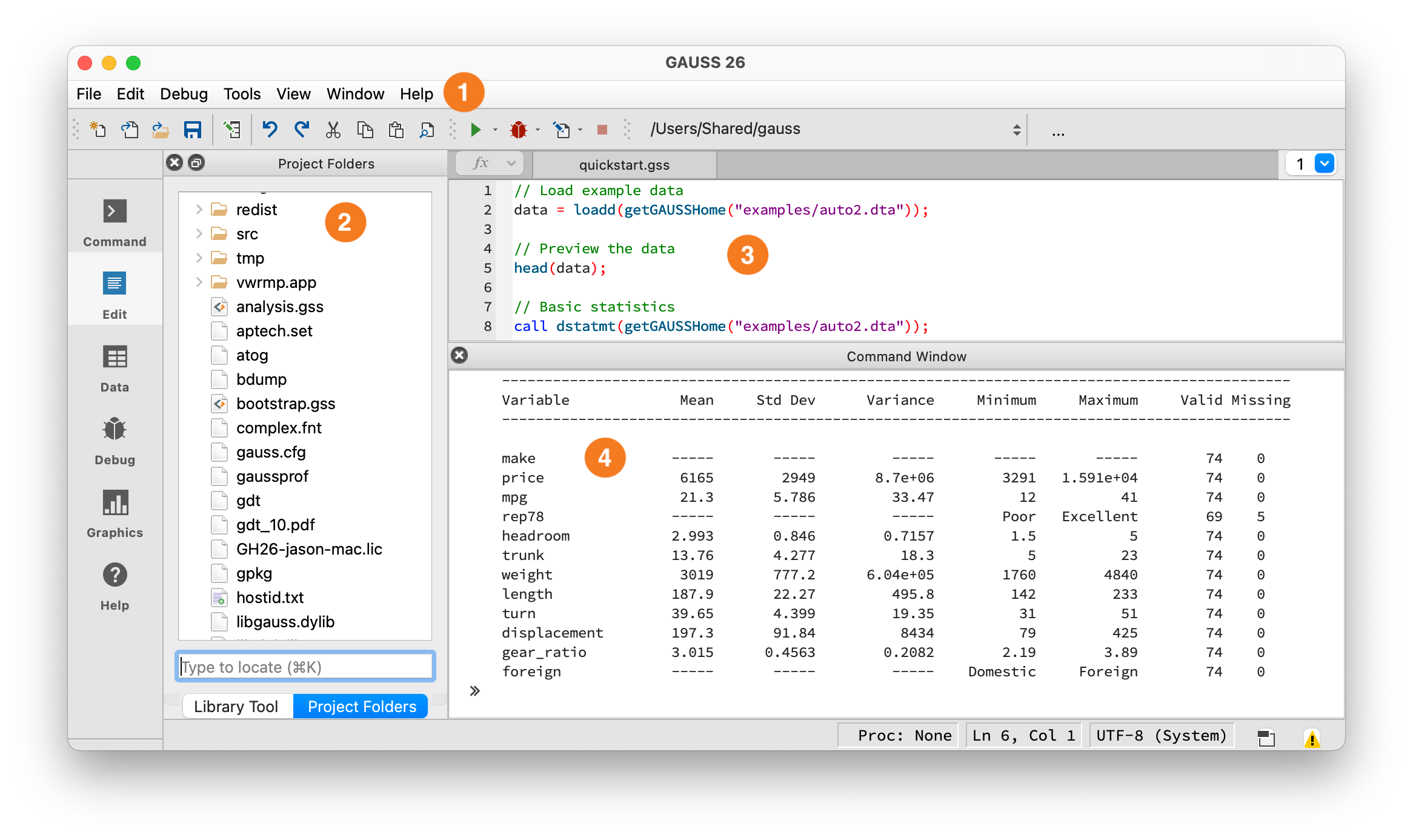
The GAUSS IDE workspace.#
① Toolbar — Shows your current working directory and the Run button (green arrow). Click it or press F5 to execute. ② Project Folders — File browser, similar to Stata’s file navigator. ③ Editor — Write programs here, similar to Stata’s Do-file Editor. ④ Command Window — Output appears here, similar to Stata’s Results window. You can also type single lines at the >> prompt.
Key Syntax Differences#
Before diving in, here are a few syntax rules that apply to all GAUSS code:
Semicolons are required. Every GAUSS statement ends with a semicolon ;. This includes block-closing keywords like endfor;, endif;, and endo;. Forgetting a semicolon causes a syntax error.
// Every statement ends with a semicolon
x = 5;
print x;
String operators use a $ prefix. GAUSS uses separate operators for string operations. The most common are:
Operator |
Purpose |
|---|---|
|
Concatenate two strings. |
|
Vertically concatenate strings into a list. |
// Build a file path
fname = getGAUSSHome() $+ "examples/auto2.dta";

// Build a list of variable names (like Stata's varlist)
vars = "mpg" $| "weight" $| "price";
Multiple datasets in memory. Unlike Stata, GAUSS does not have a single active dataset. You can load multiple datasets into separate variables and use them all at once.
Data Storage#
GAUSS stores data in matrices, string arrays, and dataframes.
Reference |
GAUSS |
Stata |
|---|---|---|
Data structure |
Dataframe or matrix |
Data set |
Series of data |
Column |
Variable |
Single occurrence |
Row |
Observation |
Missing Values |
|
|
What is a GAUSS dataframe?#
A GAUSS dataframe stores data in rows and columns like a Stata dataset, but carries type information (string, numeric, category, date) that estimation functions use automatically — for example, olsmt() creates dummy variables for categorical predictors and labels output with variable names.
The key difference from Stata: since GAUSS can hold multiple datasets at once, you always specify which dataframe a variable belongs to. Reference variables by name or column number:
// By name (the . means "all rows")
auto2[., "mpg"];

// By column number
auto2[., 4];

// A specific row
auto2[4, .];
Data Input/Output#
Constructing a dataframe from values#
In Stata, the input statement is used to build datasets from specified values and column names:
input  x y
1 2
3 4
5 6
end
In GAUSS, a dataframe can be created from a manually entered matrix and variable names using the asDF() procedure:
// Create a 3 x 2 matrix
mat = { 1 2,
        3 4,
        5 6 };

// Convert matrix to a dataframe
// and name the first column "X"
// and the second column "Y"
df = asDF(mat, "X", "Y");
Reading external datasets#
In Stata, different commands are needed for different file types — use for .dta, import delimited for CSV, import excel for spreadsheets — and each requires clear to replace the current dataset:
import delimited "tips2.csv", clear
In GAUSS, the loadd() procedure handles all common formats (CSV, Excel, Stata, SAS, SPSS, HDF5) with the same syntax, and there is no need to clear — you can have multiple datasets loaded at once:
// Get the full file path to the example dataset
fname = getGAUSSHome("examples/auto2.dta");

// Load all variables, auto-detecting their types
auto2 = loadd(fname);
To load only specific variables, use a formula string with + to list the ones you want:
// Load only three variables from tips2.csv
tips2 = loadd(getGAUSSHome("examples/tips2.csv"), "total_bill + tip + sex");
Note
Most examples below use auto2 and tips2. To run them all in order, load both datasets first:
auto2 = loadd(getGAUSSHome("examples/auto2.dta"));
tips2 = loadd(getGAUSSHome("examples/tips2.csv"));
GAUSS auto-detects variable types in most cases. If you need to override the type — most commonly for dates in non-standard formats — use the date(), cat(), or str() keywords in the formula string:
// Load ‘Date’ as a date variable (the $ indicates it is stored as a string in the file)
yellowstone = loadd(getGAUSSHome("examples/yellowstone.csv"), "Visits + HighTemp + date($Date)");
Formula string quick reference: GAUSS uses formula strings in several contexts. The syntax varies slightly:
For a complete guide to formula strings and data import options, see Programmatic Data Import.
Interactively loading data#
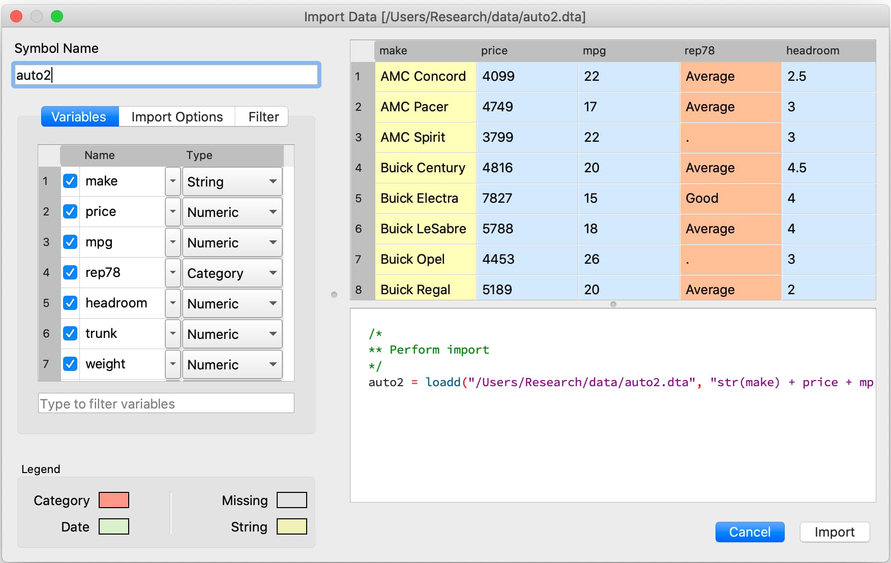
The GAUSS Data Import window is a completely interactive environment for loading data and performing preliminary data cleaning. It can be used to:
Select variables and change types.
Select observations by range or logic filtering.
Manage date formats and category labels.
Preview data.
Like Stata’s menu-driven import, the Data Import window auto-generates reusable code:
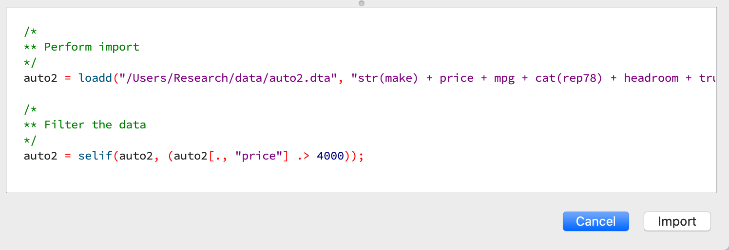
You can open the Data Import window in three ways:
Select File > Import Data from the main GAUSS menu bar.
From the Project Folders window:
Double-click on the name of the data file.
Right-click the file and select Import Data.
A complete guide to interactively loading data is available in the GAUSS Data Management guide.
Viewing Data#
View data in GAUSS with the Data Editor, a floating Symbols Editor (Ctrl+E), or by printing to the Command Window.
Print rows to screen with indexing (like Stata’s list):
// First 5 rows, all columns
auto2[1:5, .];

// First 5 rows, one variable
auto2[1:5, "mpg"];
Or use head() and tail() for a quick preview. Pass an optional row count (default is 5):
head(auto2[., "make" "price" "mpg"]);
         make            price              mpg
  AMC Concord        4099.0000        22.000000
    AMC Pacer        4749.0000        17.000000
   AMC Spirit        3799.0000        22.000000
Buick Century        4816.0000        20.000000
Buick Electra        7827.0000        15.000000
Data Operations#
Indexing matrices and dataframes#
GAUSS uses square brackets [] for indexing matrices. The indices are listed row first, then column, with a comma separating the two. For example, to index the element in the 3rd row and 7th column of the matrix x, we use:
x[3, 7];
To select a range of columns or rows with numeric indices, GAUSS uses the : operator:
x[3:6, 7];
GAUSS also allows you to use variable names in a dataframe for indexing. As an example, if we want to access the 3rd observation of the variable mpg in the auto2 dataframe, we use:
auto2[3, "mpg"];
You can also select multiple variables using a space separated list:
auto2[3, "mpg" "make"];
Finally, GAUSS allows you index an entire column or row using the . operator. For example, to see all observations of the variable mpg in the auto2 dataframe, we use:
auto2[., "mpg"];
Operations on variables#
In Stata, generate and replace are required to either transform existing variables or generate new variables using existing variables:
replace total_bill = total_bill - 2
generate new_bill  = total_bill / 2
In GAUSS, use standard operators and assign back to the dataframe column:
// Replace: subtract 2 from total_bill
tips2[., "total_bill"] = tips2[., "total_bill"] - 2;
To create a new variable (Stata’s generate), use insertcols() to insert a named column at a specific position:
// Generate: create new_bill as total_bill / 2, inserted after total_bill
new_col = dfname(tips2[., "total_bill"] / 2, "new_bill");
tips2 = insertcols(tips2, "total_bill", new_col);
Or append to the end with ~ (horizontal concatenation):
tips2 = tips2 ~ dfname(tips2[., "total_bill"] / 2, "new_bill");
Matrix operations#
Common Matrix Operators
Description |
GAUSS |
Stata |
|---|---|---|
Matrix multiply |
|
|
Solve system of linear equations |
|
|
Kronecker product |
|
|
Matrix transpose |
|
|
When dealing with matrices, it is important to distinguish matrix operations from element-by-element operations. In Stata, element-by-element operations are specified with a colon :. In GAUSS, element-by-element operations are specified by a dot ..
Element-by-element (ExE) Operators
Description |
GAUSS |
Stata |
|---|---|---|
Element-by-element multiply |
|
|
Element-by-element divide |
|
|
Element-by-element exponentiation |
|
|
Element-by-element addition |
|
|
Element-by-element subtraction |
|
|
For more on matrix operations in GAUSS:
Filtering#
In Stata, data is filtered using an if clause when using other commands. For example, to keep all observations where total_bill is greater than 10 we use:
keep if total_bill > 10
In GAUSS this can be done interactively with the Data Management Tool:
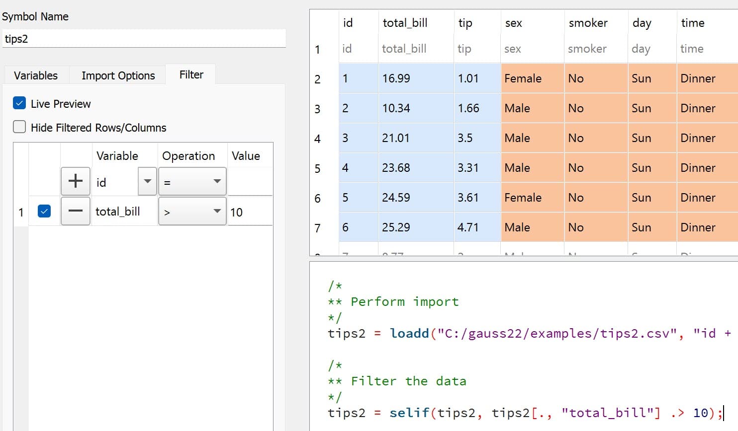
Programmatically, use selif(). The .> operator is an element-by-element comparison — the dot means “compare each row individually”:
tips2 = selif(tips2, tips2[., "total_bill"] .> 10);
More information about filtering data can be found in:
The Interactive Data Cleaning section of the Data Management Guide.
Selection of data#
Stata allows you to select, drop, or rename columns using command line keywords:
keep sex total_bill tip

drop sex

rename total_bill total_bill_2
In GAUSS, the same can be done using the Data Management pane.
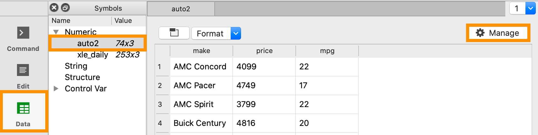
To open the Data Management pane:
Double-click the name of the dataframe in the Symbols window on the Data page.
Click the Manage button with the cog icon on the top right of the open Symbol Editor window.
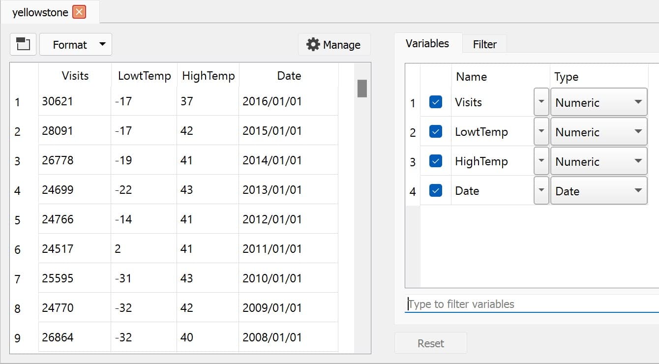
Select columns from a dataframe#
Columns can be selected or removed from the dataframe using the Variables list.
If a variable has a check box next to the name of the variables it is included in the dataframe.
To clear the variable from the dataframe clear the check box next to the variable name.
These changes will not be made until you click Apply.
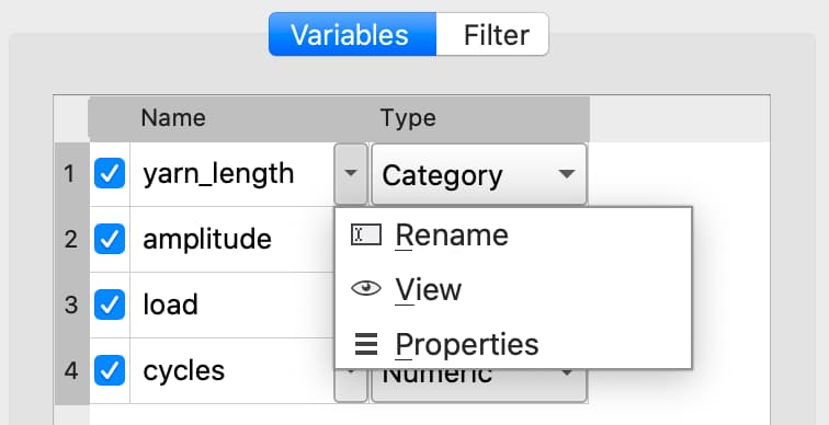
Changing variable names#
Variable names can also be changed from the Variables list.
Double-click the dataframe you want to modify in the Symbols pane of the Data page.
Click the Manage button at the top right of the open Symbol Editor.
Click downward pointing triangle button to the right of the name of the variable name you want to change and select Rename.
Enter the new name in the Name text box.
These changes will not be made until you click Apply.
GAUSS also offers programmatic options for selecting data and changing variable names:
// Keep only 'total_bill' 'tip' and 'sex'
tips2 = tips2[., "total_bill" "tip" "sex"];

// Drop sex variable
tips2 = delcols(tips2, "sex");

// Rename variable 'total_bill' to 'total_bill_2'
tips2 = dfname(tips2, "total_bill_2", "total_bill");
Sorting#
In Stata the sort command is used for sorting data:
sort sex total_bill
In GAUSS, use sortc():
tips2 = sortc(tips2, "sex" $| "total_bill");
Collapsing / aggregating by group#
In Stata, collapse computes group-level statistics:
collapse (mean) tip (sum) total_bill, by(day)
In GAUSS, use aggregate():
// Mean of all numeric columns by 'day'
tips_mean = aggregate(tips2, "mean", "day");

// Aggregate by multiple grouping variables
tips_grp = aggregate(tips2, "max", "day" $| "time");
Supported methods: "mean", "median", "sum", "min", "max", "sd", "variance", "mode".
Reshaping: wide to long and long to wide#
In Stata, reshape converts between wide and long formats:
reshape long Cars_, i(Years) j(type) string
reshape wide num_nests, i(region) j(year)
In GAUSS, use dfLonger() (wide → long) and dfWider() (long → wide):
// Wide to long
df_wide = loadd(getGAUSSHome("examples/tiny_car_panel.csv"));
columns = "Cars_compact" $| "Cars_truck" $| "Cars_SUV";
df_long = dfLonger(df_wide, columns, "type", "count");
// Long to wide
df_long = loadd(getGAUSSHome("examples/eagle_nests_long.csv"));
df_wide = dfWider(df_long, "year", "num_nests");
By-group operations#
Stata’s bysort runs commands group by group:
bysort day: summarize tip
In GAUSS, use aggregate() with a grouping column:
// Mean tip by day (Stata's bysort day: summarize tip)
tip_by_day = aggregate(tips2[., "day" "tip"], "mean", "day");
Estimation#
OLS Regression#
In Stata, linear regression is run using the regress command:
regress price mpg weight
In GAUSS, OLS is run using olsmt(). GAUSS estimation functions use formula strings to specify models: the ~ separates the dependent variable (left) from predictors (right).
Results are stored in a structure — GAUSS’s equivalent of Stata’s e() results. You declare the structure type before calling the function, then access members with dot notation. The pattern is the same for every estimation function: declare, call, access with dots.
// Load data
auto2 = loadd(getGAUSSHome("examples/auto2.dta"));

// Declare output structure (like Stata's e() but typed)
struct olsmtOut out;

// Run OLS: price on mpg and weight
out = olsmt(auto2, "price ~ mpg + weight");
This prints a familiar-looking regression table:
Ordinary Least Squares
====================================================================================
Valid cases:                       74          Dependent variable:             price
Missing cases:                      0          Deletion method:                 None
Total SS:                    6.35e+08          Degrees of freedom:                71
R-squared:                      0.293          Rbar-squared:                   0.273
Residual SS:                 4.49e+08          Std. err of est:             2.51e+03
F(2,71):                         14.7          Probability of F:            4.42e-06
====================================================================================
                            Standard                    Prob       Lower       Upper
Variable        Estimate       Error     t-value        >|t|       Bound       Bound
------------------------------------------------------------------------------------

CONSTANT          1946.1        3597     0.54102     0.59019     -5104.1      8996.3
mpg              -49.512      86.156    -0.57468     0.56732     -218.38      119.35
weight            1.7466     0.64135      2.7232   0.0081298     0.48951      3.0036
====================================================================================
To access individual results programmatically — the equivalent of Stata’s _b[mpg] and _se[mpg] — use the output structure members:
print out.b;        // Coefficient estimates
print out.stderr;   // Standard errors
print out.rsq;      // R-squared
For robust or clustered standard errors (Stata’s , robust and , cluster()), pass an olsmtControl structure — see the olsmt() reference for details.
Logistic Regression#
In Stata, logistic regression is run using the logit command:
logit foreign mpg weight
In GAUSS, this is done using glm() with the "binomial" distribution:
struct glmOut gOut;
gOut = glm(auto2, "foreign ~ mpg + weight", "binomial");
This prints:
Generalized Linear Model
===================================================================
Valid cases:              74           Dependent variable:  foreign
Degrees of freedom:       71           Distribution        binomial
Deviance:               54.4           Link function:         logit
===================================================================
                                   Standard                    Prob
Variable               Estimate       Error     z-value        >|z|
-------------------------------------------------------------------

CONSTANT                 13.708      4.5187      3.0337   0.0024158
mpg                    -0.16859    0.091917     -1.8341    0.066637
weight               -0.0039067   0.0010116     -3.8618  0.00011253
===================================================================
Descriptive Statistics#
In Stata, summarize provides descriptive statistics:
summarize price mpg weight
In GAUSS, this is done using dstatmt():
call dstatmt(auto2[., "price" "mpg" "weight"]);
This prints:
----------------------------------------------------------------------------------------
Variable        Mean     Std Dev      Variance     Minimum     Maximum     Valid Missing
----------------------------------------------------------------------------------------

price           6165        2949       8.7e+06        3291   1.591e+04        74    0
mpg             21.3       5.786         33.47          12          41        74    0
weight          3019       777.2      6.04e+05        1760        4840        74    0
See also
Functions olsmt(), glm(), quantileFit(), dstatmt(), frequency()
For more fully worked estimation examples, see the Econometrics blog.
Loops and Control Flow#
Loops#
In Stata, loops are written using forvalues and foreach:
forvalues i = 1/5 {
    display `i'
}

foreach var of varlist mpg weight price {
    summarize `var'
}
In GAUSS, numeric loops use for and looping over items uses for with indexing:
// Numeric loop (equivalent of forvalues)
for i(1, 5, 1);
    print i;
endfor;

// Loop over a list of variable names
vars = "mpg" $| "weight" $| "price";

for i(1, rows(vars), 1);
    call dstatmt(auto2[., vars[i]]);
endfor;
GAUSS also supports do while and do until loops:
// Do while loop
j = 1;
do while j <= 5;
    print j;
    j = j + 1;
endo;
Conditional Statements#
In Stata, if/else is used for control flow in programs:
if `x' > 10 {
    display "large"
}
else {
    display "small"
}
In GAUSS:
if x > 10;
    print "large";
else;
    print "small";
endif;
Writing Procedures#
In Stata, reusable code is wrapped in programs or ado-files:
program define demean
    args varname
    quietly summarize `varname'
    replace `varname' = `varname' - r(mean)
end
In GAUSS, reusable code is written as a procedure using proc and endp. Variables inside a procedure must be declared local to avoid conflicts with the global workspace:
proc (1) = demean(x);
    local m;
    m = meanc(x);
    retp(x - m);
endp;

// Use the procedure
x_demeaned = demean(auto2[., "price"]);
The (1) after proc indicates the procedure returns one value. GAUSS procedures can return multiple values:
proc (2) = meanAndSD(x);
    retp(meanc(x), stdc(x));
endp;

// Capture both return values
{ m, s } = meanAndSD(auto2[., "price"]);
To call a procedure that returns nothing (like Stata’s program without rclass), use the call keyword:
proc (0) = printHeader(title);
    print "==================================";
    print title;
    print "==================================";
endp;

call printHeader("My Analysis");
For more on loops, string handling, and general GAUSS programming, see the Programming blog.
Date Functionality#
Creating usable dates from raw data#
In Stata, dates are imported as strings and must be manually converted and formatted:
generate date_var = date(date, "YMD")
format date_var %d.
In GAUSS, loadd() auto-detects common date formats — just use the date keyword in the formula string:
fname = getGAUSSHome("examples/yellowstone.csv");
yellowstone = loadd(fname, "Visits + LowTemp + HighTemp + date($Date)");
Creating dates from existing strings#
The GAUSS asDate() procedure works similarly to the Stata date() function and can be used to convert strings to dataframe dates.
For example, suppose we want to convert the string "2002-10-01" to a date in Stata:
generate date_var = date("2002-10-01", "YMD")
When we do this in Stata the data is displayed in the date numeric format and we have to use the format command to change the display format:
format date_var %d
In GAUSS, this is done using the asDate() procedure:
// Convert string date '2002-10-01'
// to a date variable
date_var = asDate("2002-10-01");
The asDate() procedure automatically recognizes dates in the format "YYYY-MM-DD HH:MM:SS". However, if the date is in a different format, a format string can be used:
// Convert string date '10/01/2002'
// to a date variable
date_var = asDate("10/01/2002", "%d/%m/%Y");
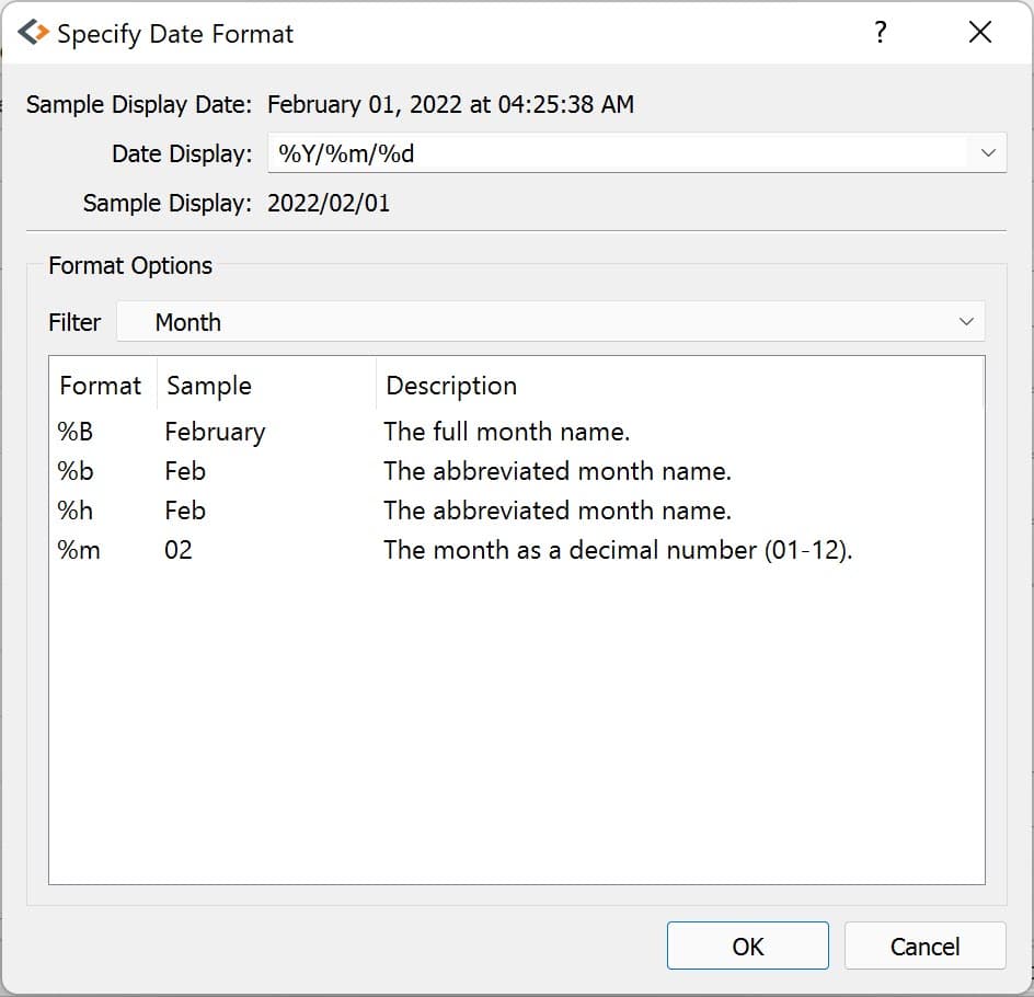
Changing the display format#
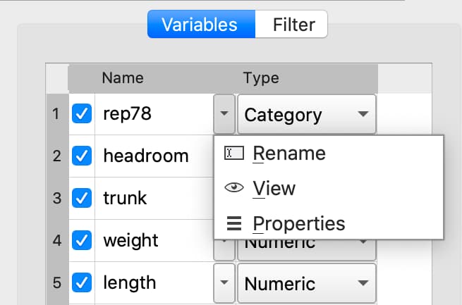
Once a date variable has been imported or created, the display format can be specified interactively using the GAUSS Data Management Tool.
The Specify Date Format dialog is accessed by selecting Properties from the variable’s dropdown:
If the variable is a date variable, the Specify Date Format window will open:
Dates can be managed programmatically using asDate():
// Convert 'Date' variable from string variable
// to date variable
yellowstone =  asdate(yellowstone, "%b-%d-%Y", "Date");
String Processing#
GAUSS has string functions similar to those in Stata. Here is a quick reference:
For example, to change the case of a string variable:
// Change time variable to uppercase
tips2[., "time"] = upper(tips2[., "time"]);

// Change sex variable to lowercase
tips2[., "sex"] = lower(tips2[., "sex"]);
Missing values#
Missing values are represented by the same dot notation, ., in both Stata and GAUSS.
This notation can be used for filtering data in Stata:
* Keep missing values
list if value_x == .

* Keep non-missing values
list if value_x != .
In GAUSS, a missing value is represented by .. To filter based on missing values, create a missing value scalar and use element-by-element comparison:
x = { 1,
      .,
      3,
      . };

// Create a missing value for comparison
mss = { . };

// Keep missing values
x_miss = selif(x, x .== mss);       // Returns: . | .

// Keep non-missing values
x_clean = selif(x, x .!= mss);      // Returns: 1 | 3
Counting, removing, and replacing missing values#
Count missing values with counts() (Stata’s count if rep78 == .):
mss = { . };
counts(auto2[., "rep78"], mss);
The dstatmt() output also includes Valid and Missing columns for each variable.
Remove rows containing missing values with packr() (drops any row with a missing value) or delif() (drops rows based on a condition):
a = { 1 .,
      . 4,
      5 6 };

packr(a);                          // Returns: 5 6 (only complete row)

mss = { . };
delif(a, a[., 2] .== mss);        // Returns rows where column 2 is not missing
Replace missing values with missrv() (like Stata’s replace a = -999 if a >= .):
missrv(a, -999); // Replaces all missing values with -999
For statistical imputation (mean, median, mode, predictive mean matching, and more), use impute().
See also
Merging#
Stata’s merge works with one dataset in memory and one on disk, creating a _merge indicator. GAUSS merges two in-memory dataframes using outerJoin() or innerJoin():
In Stata, merging two small datasets requires saving one to disk first:
merge 1:1 ID using df1
In GAUSS, both datasets stay in memory:
// Build two small dataframes
df1 = asDF("John" $| "Mary" $| "Susan" $| "Connie", "ID")
    ~ asDF(22 | 18 | 34 | 45, "Age");

df2 = asDF("John" $| "Mary" $| "Susan" $| "Tyler", "ID")
    ~ asDF("Teacher" $| "Surgeon" $| "Developer" $| "Nurse", "Occupation");

// Full outer join — keep all rows from both dataframes
df3 = outerJoin(df2, "ID", df1, "ID", "full");
    ID       Occupation              Age
  John          Teacher        22.000000
  Mary          Surgeon        18.000000
 Susan        Developer        34.000000
 Tyler            Nurse                .
Connie                .        45.000000
Omit "full" to keep only rows that match the left dataframe:
df3 = outerJoin(df2, "ID", df1, "ID");
What’s Next?#
Command Reference — Browse all 1,000+ built-in functions
Data Management — Loading, cleaning, and reshaping data
Textbook Examples — Worked examples from Greene (Econometric Analysis) and Brooks (Introductory Econometrics for Finance)
Econometrics blog — Fully worked examples covering regression, panel data, hypothesis testing, and more
Time series blog — ARIMA, VAR, GARCH, cointegration, and forecasting tutorials with complete code
Panel data blog — Fixed effects, random effects, and dynamic panel models
Programming blog — Loops, string handling, data manipulation, and general GAUSS programming
saved()— Export data to CSV, Excel, or other formats (Stata’sexport)User Guide — Installing and managing add-on modules (Stata’s
ssc install)