Data Exploration#
Descriptive statistic table#
The dstatmt() procedure generates a summary table of descriptive statistics. It computes following statistics for every numeric column:
Mean
Standard deviation
Variance
Minimum
Maximum
Valid cases
Missing cases
It works directly with matrices and dataframes and will print a complete summary table to the Command window.
Example: Summary statistics from a datafile#
// Create file name with full path
file_name = getGAUSSHome("examples/fueleconomy.dat");

// Compute statistics for all variables in the dataset
// The 'call' keyword disregards return values from the function
call  dstatmt(file_name);
This prints the following results
----------------------------------------------------------------------------------------------------
Variable                    Mean     Std Dev      Variance     Minimum     Maximum     Valid Missing
----------------------------------------------------------------------------------------------------

annual_fuel_cost           2.537      0.6533        0.4267        1.05         5.7       978    0
engine_displacement        3.233       1.376         1.892           1         8.4       978    0
The dstatmt() function can also be used on a subset of variables, rather than the entire dataset.
Example: Summary statistics for select variables#
// Load 'nba_ht_wt' data
fname = getGAUSSHome("examples/nba_ht_wt.xls");
nba_ht_wt = loadd(fname);

// Compute statistics for 'Height', 'Weight', and 'Age'
// The 'call' keyword disregards return values from the function
call  dstatmt(nba_ht_wt, "Height"$|"Weight"$|"Age");
This prints the following output:
----------------------------------------------------------------------------------------
Variable        Mean     Std Dev      Variance     Minimum     Maximum     Valid Missing
----------------------------------------------------------------------------------------

Height         79.07       3.454         11.93          69          87       505    0
Weight         220.7       26.64         709.9         157         290       505    0
Age            26.19       4.325         18.71          15          40       505    0
Individual descriptive statistics#
Statistic |
Matrices |
Arrays |
|---|---|---|
Mean |
||
Median |
||
Mode |
||
Quantiles |
||
Sample standard deviation |
||
Pop. Standard deviation |
||
Minimum |
||
Maximum |
||
Sum |
Example: Finding mean by column#
// Create file name with full path
fname = getGAUSShome("examples/xle_daily.xlsx");

// Load all three variables, 'Date', 'Adj Close'
// and 'Volume'.
xle_daily = loadd(fname);

// Find mean of 'Adj Close' and 'Volume'
meanc(xle_daily[., "Adj Close" "Volume"]);
The results are printed directly to screen:
68.442841
14308087.
Computing group descriptive statistics#
The aggregate() procedure finds descriptive statistics for each group in panel data. It allows an optional input to specify the name of the categorical variable to be used for grouping.
In order to be used with aggregate() data should:
Have group identifiers in the first column if the name of the categorical variable for grouping is not specified.
Be in stacked panel data format (see
dfLonger()).
If the input data is contained in a dataframe, the aggregate() procedure will output a dataframe.
The function supports the following statistics for grouping:
Mean
Median
Mode
Min
Max
Sample standard deviation
Sum
Sample variance
The aggregate() function also accepts an optional indicator input for fast computation. If fast computation is specified, the procedure will not check for missing values.
Example One: Group variable contained in first column#
In this example, the group variable is included in the first column. No categorical variable is specified for grouping.
// Create file name with full path
fname = getGAUSSHome("examples/housing.csv");

// Load three variables from 'housing' dataset
X = loadd(fname, "beds + price + size");

// Compute the median of the sales price
// and size (sq ft) by the variable in the
// first column, which is the number of bedrooms.
x_a = aggregate(X, "median");
The matrix x_a contains:
beds            price             size
   2             94.3             1060
   3            132.6           1473.5
   4              179             2000
   5           352.65             3095
Example Two: Specifying the group variable as an input#
In this example, a categorical variable name is specified for grouping.
// Load 'auto2' data
fname = getGAUSSHome("examples/auto2.dta");
auto2 = loadd(fname);

// Aggregate data using foreign column as group
aggregate(auto2[., "price" "mpg" "foreign"], "mean", "foreign");
The aggregated results are printed to the Command window:
foreign     price      mpg
Domestic  6072.423   19.827
Foreign   6384.682   24.773
Note
The aggregate() function is similar to creating pivot tables, where:
The group variable is equivalent to a pivot table row variable.
The remaining variables in x are equivalent to column variables.
The method input is equivalent to the values setting in a pivot table.
Frequency tables and plots#
One-way frequency counts#
The frequency() procedure computes a frequency count of all categories of a categorical variable.
// Load 'auto2' data
fname = getGAUSSHome("examples/auto2.dta");
auto2 = loadd(fname);

// Frequency table
frequency(auto2, "rep78");
The above code prints:
=============================================
          rep78     Count   Total %    Cum. %
=============================================

           Poor         2     2.899     2.899
           Fair         8     11.59     14.49
        Average        30     43.48     57.97
           Good        18     26.09     84.06
      Excellent        11     15.94       100
=============================================
          Total        69       100
Multiple tables can be generated by adding variables to the variable formula string using "+".
/*
** This example uses 'auto2' data
** which was previously loaded
*/

// Print frequency table of 'rep78' and 'foreign'
frequency(auto2, "rep78 + foreign");
=============================================
          rep78     Count   Total %    Cum. %
=============================================

           Poor         2     2.899     2.899
           Fair         8     11.59     14.49
        Average        30     43.48     57.97
           Good        18     26.09     84.06
      Excellent        11     15.94       100
=============================================
          Total        69       100

=============================================
        foreign     Count   Total %    Cum. %
=============================================

       Domestic        52     70.27     70.27
        Foreign        22     29.73       100
=============================================
          Total        74       100
An optional indicator input can be used with the frequency() procedure to sort the table in descending order.
/*
** This example uses 'auto2' data
** which was previously loaded
*/

// Print sorted frequency table of 'rep78'
frequency(auto2, "rep78", 1);
=============================================
          rep78     Count   Total %    Cum. %
=============================================

        Average        30     43.48     43.48
           Good        18     26.09     69.57
      Excellent        11     15.94     85.51
           Fair         8     11.59      97.1
           Poor         2     2.899       100
=============================================
          Total        69       100
As an alternative to frequency(), the counts() procedure counts the numbers of elements of a vector that fall into specified ranges and can be used to create frequency tables.
For example, to find the frequency of each category for a categorical variable, use counts() with the unique category keys as cutoffs.
/*
** Create frequency table of 'rep78'
** using counts procedure and
** auto2 data loaded in earlier example
*/
print "Frequency table of rep78:";

// Extract column labels
{ label, keyvalues } = getcollabels(auto2, "rep78");

// Get data counts using keyvalues
counts(auto2[., "rep78"], keyvalues);
Frequency table of rep78:

     2.0000000
     8.0000000
     30.000000
     18.000000
     11.000000
Frequency plots#
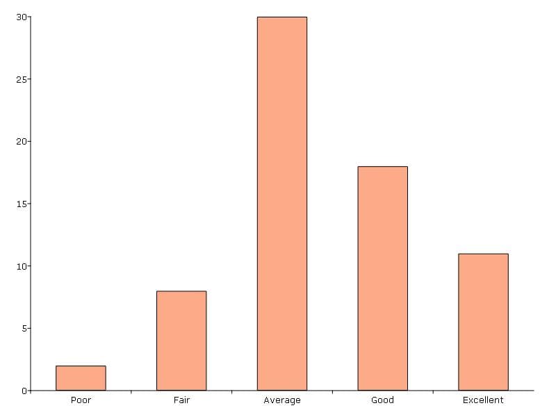
The plotFreq() procedure will compute and plot frequencies for a categorical variable. A quick plot can be generated using default formatting or an optional plotControlStructure can be used for custom formatting. An optional indicator input can be used with the plotFreq() procedure to sort the bars in descending order.
Plotting category frequency#
// Load 'auto2' data
fname = getGAUSSHome("examples/auto2.dta");
auto2 = loadd(fname);

// Frequency plot of 'rep78' categories
plotFreq(auto2, "rep78");
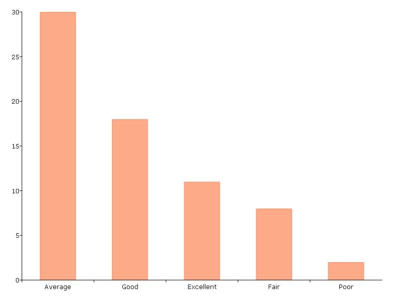
Plotting sorted frequencies#
In this example, the optional argument, sort, is used to specify that the bars should be sorted in order from most frequently to least frequently occurring.
/*
** This example uses 'auto2' data
** which was previously loaded
*/

// Sorted frequency plot of 'rep78'
plotFreq(auto2, "rep78", 1);
Plotting frequencies percentages#
In this example, the optional argument, pct_axis, is used to specify frequency percentages should be plotted. Note the optional argument, sort, must still be specified because optional arguments must be specified in order.
/*
** This example uses 'auto2' data
** which was previously loaded
*/

// Unsorted, percent frequency plot of 'rep78'
plotFreq(auto2, "rep78", 0, 1);

Plotting by groups#
In this example, the by keyword is used for plotting categorical frequencies by groups. Specifically, the
// Load dataset
tips2 = loadd("tips2.csv");

// Create a frequency plot of visits per day
// for each category of smoker (Yes, or No).
plotFreq(tips2, "day + by(smoker)");

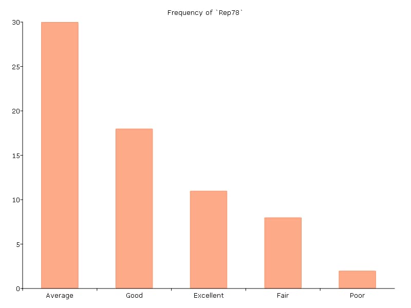
Customizing frequency plots#
In the next example, a plotControl structure is used to add a title to the sorted frequency plot.
/*
** This example uses 'auto2' data
** which was previously loaded
*/

// Declare plotControl structure
struct plotControl myPlt;
myPlt = plotGetDefaults("bar");

// Set title
plotSetTitle(&myPlt, "Frequency of `Rep78`");

// Sorted frequency plot of 'rep78' with custom format
// using myPlt structure
plotFreq(myPlt, auto2, "rep78", 1);
Two-way tables#
The tabulate() procedure generates two-way tables and returns the counts as a dataframe.
Basic tabulation with the tabulate() procedure requires:
A dataframe or filename input.
A formula string to specify which variables to include in the table.
The formula string specifies the row variable on the left-hand side of the tilde and column variables on the right-hand side.
// Load 'tips2' dataset
fname = getGAUSSHome("examples/tips2.dta");
tips  = loadd(fname);

// Create two-way table with sex in rows
// and smoking status in columns
call tabulate(tips, "sex ~ smoker");
============================================================
      sex                   smoker                 Total
============================================================
                      No            Yes


   Female             55             33               88
     Male             99             60              159

    Total            154             93              247
============================================================
Multiple tables can be generated by including additional right-hand side column variables using "+".
/*
** This example uses 'tips' data
** which was previously loaded
*/

// Generate separate tables for sex vs smoker
// and sex vs time
call tabulate(tips, "sex ~ smoker + time");
 ============================================================
           sex                   smoker                 Total
 ============================================================
                          No            Yes


       Female             55             33               88
         Male             99             60              159

        Total            154             93              247
 ============================================================
          sex                    time                  Total
 ============================================================
                       Lunch         Dinner


       Female             35             53               88
         Male             33            126              159

        Total             68            179              247
============================================================
An optional tabControl structure input can be used for advanced options including. An instance of the tabControl structure, tCtl, includes the following members:
Member |
Description |
|---|---|
tCtl.exclude |
String, the categories to be excluded from table counts. Totals will not include observations in excluded categories. |
tCtl.UnusedLevels |
Scalar, indicates whether to include unused levels in table. Set to 0 to remove unused levels from the table. Default = 1. |
tCtl.rowPercent |
Scalar, indicates whether to report row percentages. Set to 1 to report row percentages. Default = 0. |
tCtl.columnPercent |
Scalar, indicates whether to report column percentages. Set to 1 to report column percentages. Default = 0. |
Dropping unused categories from the table#
Consider the following two-way frequency table:
/*
** This example uses 'tips' data
** which was previously loaded
*/

// Take the first 50 observations of
// previously loaded 'tips' data as a sample
tips_subset = tips[1:50, .];

// Compute and print the frequency table
call tabulate(tips_subset, "day ~ smoker");
============================================================
            day                   smoker               Total
============================================================
                            No            Yes


           Thur              0              0              0
            Fri              0              0              0
            Sat             23              0             23
            Sun             27              0             27

          Total             50              0             50
============================================================
The unusedCategories member of the tabControl structure can be used to drop the unused day categories, Thur and Fri, as well as theunused Yes smoker category from the table.
/*
** This example uses 'tips' data
** which was previously loaded
*/

// Declare an instance of the
// tabControl structure
// and fill with defaults
struct tabControl tbctl;
tbctl = tabControlCreate();

// Supress unrepresented categories
// by setting unusedLevels member to 0
tbctl.unusedLevels = 0;

// Compute and print the frequency table
call tabulate(tips_subset, "day ~ smoker", tbctl);
The table no longer includes the unused categories from the table.
=============================================
            day         smoker          Total
=============================================
                            No


            Sat             23             23
            Sun             27             27

          Total             50             50
=============================================
Excluding specified categories from the table#
Specific categories can be excluding from the table using the exclude member of the tabControl structure. This input is a string array input which must include the variable name and the associated category, separated by a ":".
/*
** This example uses 'tips' data
** which was previously loaded
*/

// Declare an instance of the
// tabControl structure
// and fill with defaults
struct tabControl tbctl;
tbctl = tabControlCreate();

// Exclude non-smokers from the table
tbctl.exclude = "smoker:No";

// Compute and print the frequency table
call tabulate(tips, "day ~ smoker", tbctl);
=============================================
            day         smoker          Total
=============================================
                          Yes


           Thur             17             17
            Fri             15             15
            Sat             42             42
            Sun             19             19

          Total             93             93
=============================================
Reporting row and column percentages#
Row percentages can be reported by setting the rowPercent member of the tabControl structure to 1.
/*
** This example uses 'tips' data
** which was previously loaded
*/

// Declare an instance of the
// tabControl structure
// and fill with defaults
struct tabControl tbctl;
tbctl = tabControlCreate();

// Report row percentages
// by setting rowPercent member to 1
tbctl.rowPercent = 1;

// Compute and print the frequency table
call tabulate(tips, "day ~ smoker", tbctl);
============================================================
            day                   smoker               Total
============================================================
                            No            Yes


           Thur           73.0           27.0            100
            Fri           21.1           78.9            100
            Sat           52.8           47.2            100
            Sun           75.0           25.0            100

============================================================
Similarly, the columnPercent member of the tabControl structure can be used to report column percentages.
/*
** This example uses 'tips' data
** which was previously loaded
*/

// Declare an instance of the
// tabControl structure
// and fill with defaults
struct tabControl tbctl;
tbctl = tabControlCreate();

// Report row percentages
// by setting rowPercent member to 1
tbctl.columnPercent = 1;

// Compute and print the frequency table
call tabulate(tips, "day ~ smoker", tbctl);
=============================================
                 day                   smoker
=============================================
                            No            Yes


           Thur           29.9           18.3
            Fri            2.6           16.1
            Sat           30.5           45.2
            Sun           37.0           20.4
          Total            100            100

=============================================
Table reports column percentages.
Table reports row percentages. Associations and correlations ———————————-
Computing correlations#
Two GAUSS functions are available for computing correlations of a sample:
Function |
Description |
|---|---|
Computes the sample correlation using a moment matrix as the input. |
|
Computes the sample correlation using a data matrix as the input. |
Example:Finding correlation of height and weight in NBA players#
// Load 'nba_ht_wt' data
fname = getGAUSSHome("examples/nba_ht_wt.xls");
nba_ht_wt = loadd(fname);


// Calculate correlation of height and weight
corrxs(nba_ht_wt[., "Height" "Weight"]);
This prints the correlations to screen:
    Height           Weight
 1.0000000       0.82071923
0.82071923        1.0000000
Finding variance-covariance#
Two GAUSS functions are available for computing covariances of a sample:
Function |
Description |
|---|---|
Computes the variance-covariance matrix using a moment matrix as the input. |
|
Computes the variance-covariance matrix using a data matrix as the input. |
Example: Finding variance/covariance of height and weight in NBA players#
// Load 'nba_ht_wt' data
fname = getGAUSSHome("examples/nba_ht_wt.xls");
nba_ht_wt = loadd(fname);


// Calculate variance-covariance
// of height and weight
varCovxs(nba_ht_wt[., "Height" "Weight"]);
This prints the following variance/covariance matrix:
11.930245        75.527346
75.527346        709.85534
Exploratory data visualizations#
GAUSS graphics are powerful enough to generate custom, publication quality plots but are equally useful for generating quick exploratory plots. Supported plots include:
XY plots.
Surface plots.
Time-series plots.
Box plots.
Histograms.
Log-Log, Log-X, and Log-Y plots.
Bar plots.
Contour plots.
Area plots.
This section offers an introduction to a selection of visualization tools for preliminary data exploration. It is not meant to act as a comprehensive GAUSS graphics guide.
Histograms#
Histograms of data can be plotted using one of three functions:
The
plotHist()function which computes and graphs a frequency histogram for a given vector of data.The
plotHistP()function which computes and graphs a percent frequency histogram for a given vector of data..The
plotHistF()function which graphs a histogram given vector of frequency counts.
Note
These functions do not currently utilize the categorical labels and plotFreq() is recommended for categorical variables with labels.
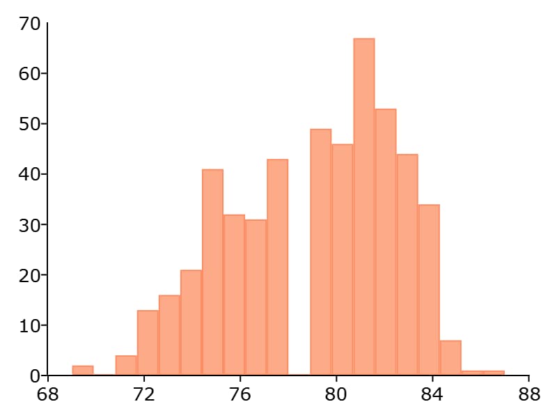
Frequency histograms#
The plotHist() function requires two inputs, a vector of data and the number of bins.
// Load 'nba_ht_wt' data
fname = getGAUSSHome("examples/nba_ht_wt.xls");
nba_ht_wt = loadd(fname);

// Plot histogram of heights with 15 bins
plotHist(nba_ht_wt[., "Height"], 20);
Percent frequency histograms#
The plotHistP() function also requires two inputs, a vector of data and the number of bins.
/*
** This example uses 'nba_ht_wt' data
** which was previously loaded
*/

// Plot histogram of heights with 15 bins
plotHistP(nba_ht_wt[., "Height"], 20);

Scatter plots#
The plotScatter() function creates a quick scatter plot using either:
A x and y input.
A dataframe name and formula string specifying x and y.
Using a dataframe with a formula string, will result in automatic labeling of the x and y axis. To add additional custom formatting, use the plotControl structure.
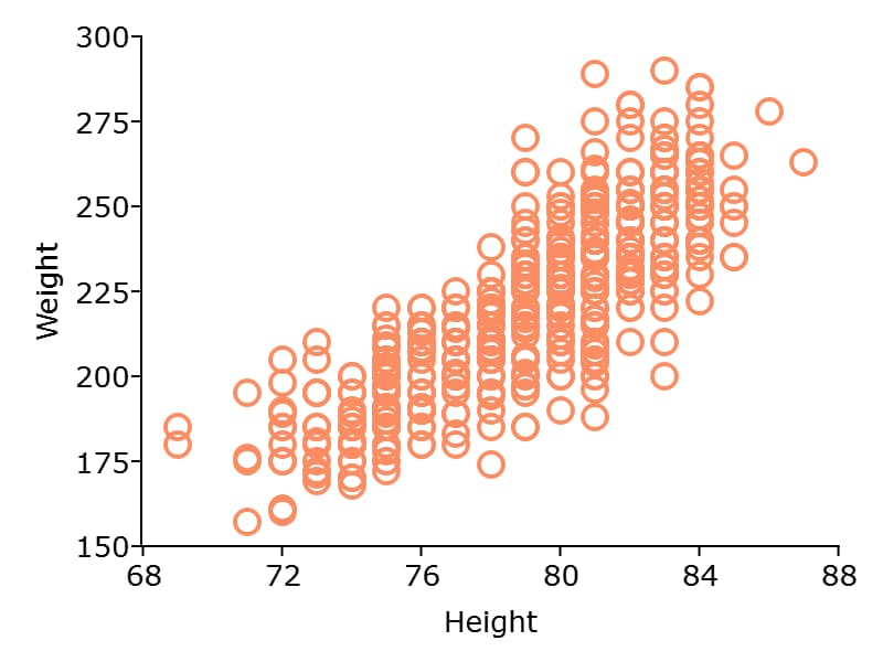
Example: Scatter plots with formula strings#
// Load 'nba_ht_wt' data
fname = getGAUSSHome("examples/nba_ht_wt.xls");
nba_ht_wt = loadd(fname);

// Plot height and weight
plotScatter(nba_ht_wt, "Weight ~ Height");
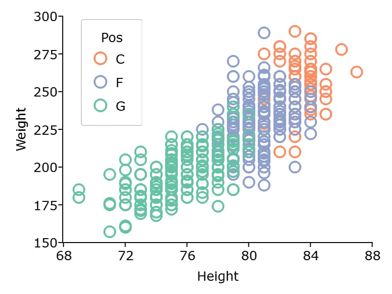
The scatter points can be color coded by categories using the "by" keyword in the formula string.
/*
** This example uses 'nba_ht_wt' data
** which was previously loaded
*/

// Plot height and weight
// color coded by 'position'
plotScatter(nba_ht_wt, "Weight ~ Height + by(Pos)");
Box plots#
The plotBox() procedure graphs data using the box graph percentile method. The procedure allows for three different sets of inputs:
A dataframe and a formula string.
A list group numbers or string labels corresponding to each column data and a data matrix.
A categorical dataframe vector and a data matrix.
Example: Using a dataframe and formula string to generate a box plot#
// Load 'auto2' data
fname = getGAUSSHome("examples/auto2.dta");
auto2 = loadd(fname);

// Draw a box plot with 'mpg' data for each of
// the two categories in 'foreign'
plotBox(auto2, "mpg ~ foreign");

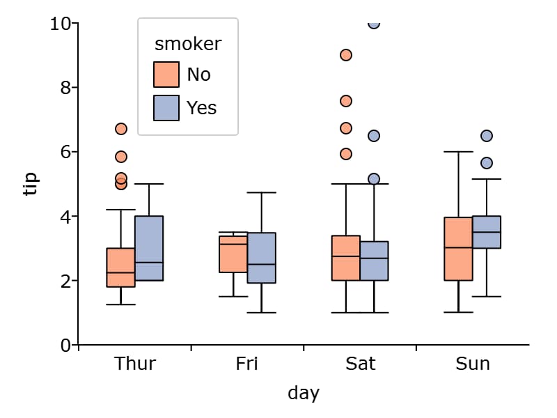
Like the scatter plot, box plots can be split by categories using the "by" keyword in the formula string.
// Import data
fname = getGAUSSHome("examples/tips2.dta");
tips = loadd(fname);

// Draw a box with 'tip' data for each day,
// split by whether 'smoker' equals yes or no.
plotBox(tips, "tip ~ day + by(smoker)");
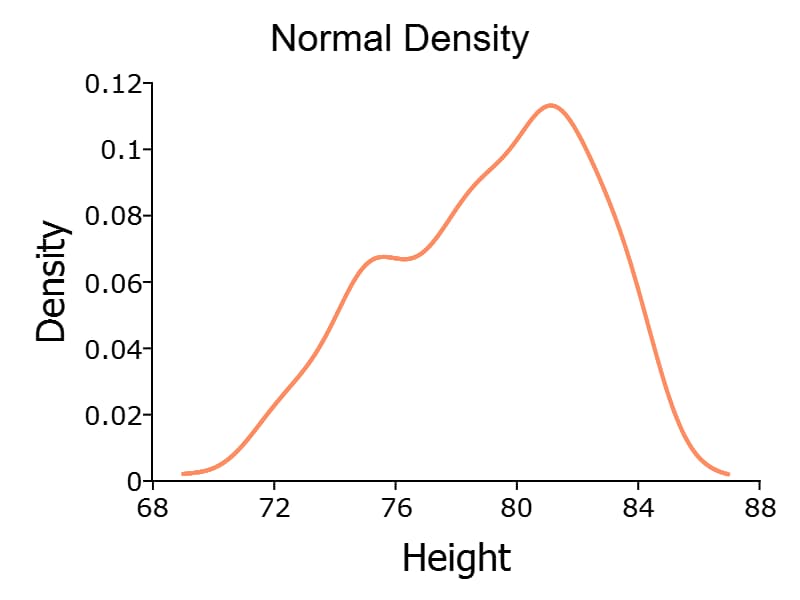
Kernel Density Plots#
The kernelDensity() procedure computes and plots kernel densities, with support for 13 different kernels:
Normal (default).
Epanechnikov.
Biweight.
Triangular.
Rectangular.
Truncated normal.
Parzen.
Cosine.
Triweight.
Tricube.
Logistic.
Sigmoid.
Silverman.
// Load 'nba_ht_wt' data
fname = getGAUSSHome("examples/nba_ht_wt.xls");
nba_ht_wt = loadd(fname);

// Plot kernel density using normal kernel
call kerneldensity(nba_ht_wt, "Height");
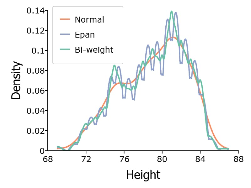
Multiple kernels can be compared in a single plot using the optional kernel input.
/*
** This example uses 'nba_ht_wt' data
** which was previously loaded
*/

// Specify kernels to compute
// 1           Normal
// 2           Epanechnikov
// 3           Biweight
kernels = { 1, 2, 3};

// Plot kernel density using normal kernel
call kerneldensity(nba_ht_wt, "Height", kernels);