Data Cleaning#
Interactive Data Cleaning#
Interactive data cleaning can be performed in the Data Import window before import, or in a GAUSS Symbol Editor after it is loaded.
This section will show how to clean data using the Data Management pane of a Symbol Editor. Most actions will be the same in the Data Import window. See Interactive Data Import
The Data Management pane#
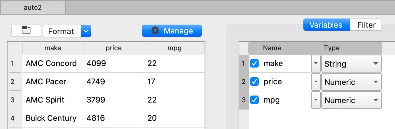
The Data Management pane contains:
The Filter tab that allows you to select observations based on a variety of criteria.
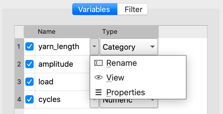
- The Variables tab that allows you to:
Select or remove variables.
Rename variables.
Change variable types.
Manage category labels and order.
Change date display formats.
Open the Data Management pane#
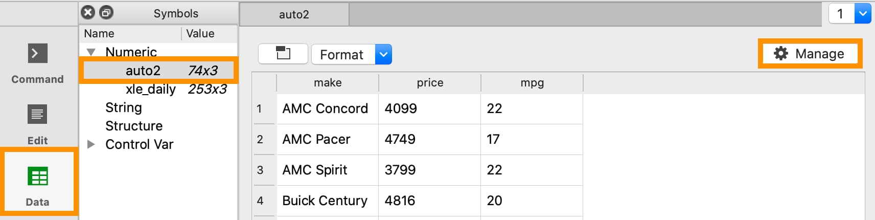
To open the Data Management pane for an in-memory dataframe:
Double-click the name of the dataframe in the Symbols window on the Data page.
Click the Manage button with the cog icon on the top right of the open Symbol Editor window.
Missing values#
Missing values are represented by a . for data loaded into GAUSS.
Remove observations with missing values interactively#
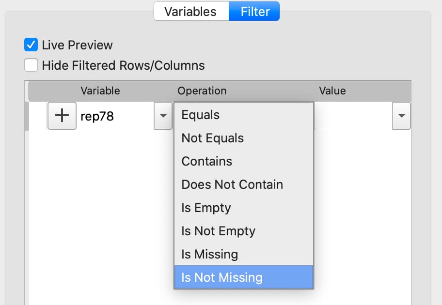
Select the variable to filter on from the Variable name drop-down list on the Filter tab.
Select Is Not Missing from the Operation drop-down list.
Click the
+button to add the filter.
All observations where the selected variable contains a missing value will be grayed out in the Data Preview window, indicating which observations will be imported.
You can click Apply or continue to create more filters.
Data organization#
Changing variable names#
Double-click the dataframe you want to modify in the Symbols pane of the Data page.
Click the Manage button at the top right of the open Symbol Editor.
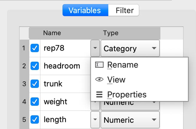
Click downward pointing triangle button to the right of the name of the variable name you want to change and select Rename.
Enter the new name in the Name text box.
These changes will not be made until you click Apply.
Deleting columns from a matrix#
Clear the check box next to the name of the variables you want to remove from the data.
These changes will not be made until you click Apply.
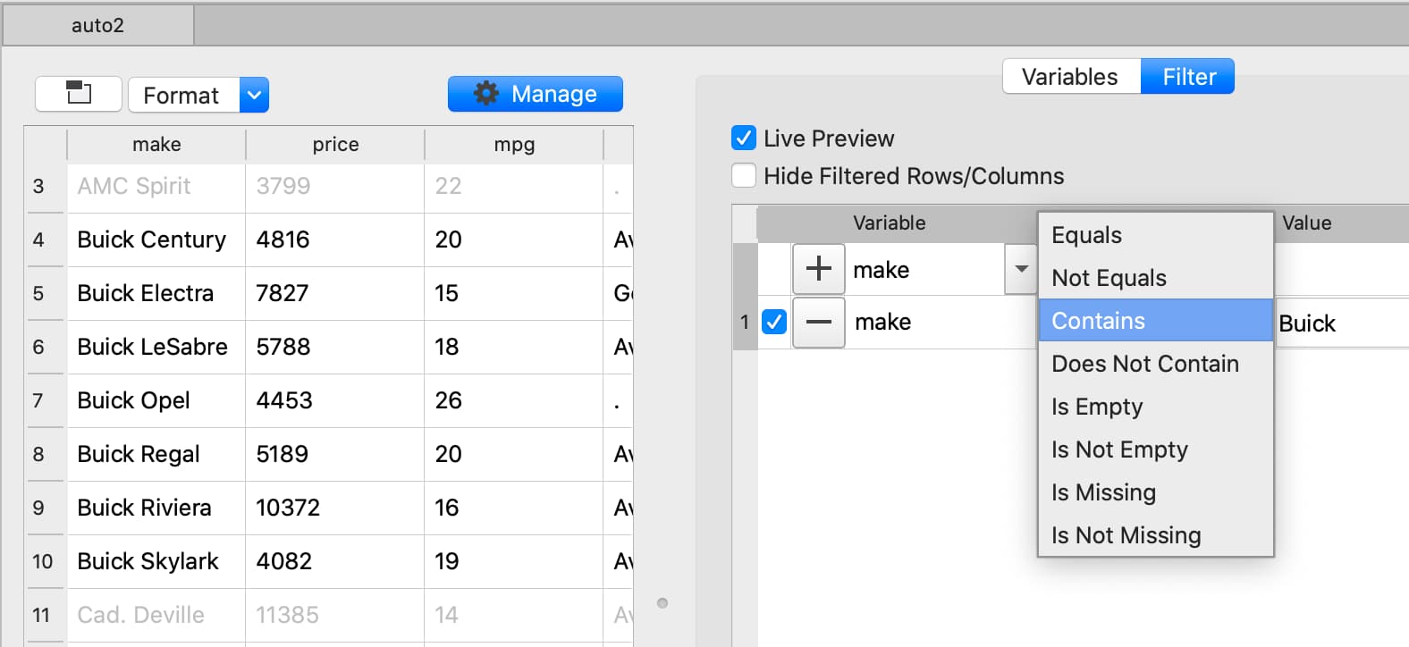
Filtering observations of a dataframe#
The Data Management pane provides the following options for filtering dataframes.
Data type |
Filter options |
Data type |
Filter options |
|---|---|---|---|
Numeric and Date |
String and Category |
||
= |
Equals |
||
!= |
Not Equals |
||
< |
Contains |
||
<= |
Does not Contain |
||
> |
Is Empty |
||
>= |
Is not Empty |
||
Is Missing |
Is Missing |
||
Is Not Missing |
Is Not Missing |
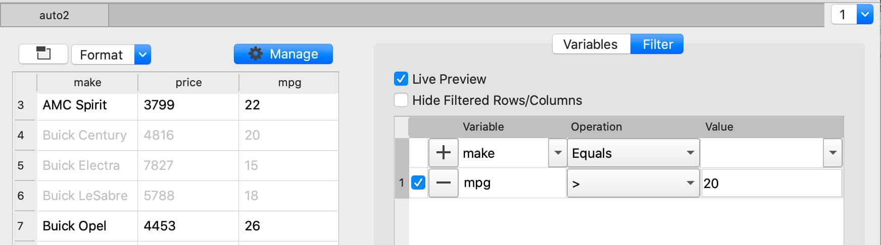
To implement any of these filtering options:
Select the variable to filter on from the Variable name drop-down list on the Filter tab.
Select the desired operation from the Operation drop-down list.
Depending on the operation, either enter or select a value in the Value combo box.
Click the
+button to add the filter.Either Apply your changes or add another filter.
Filter based on partial string match#
Filter based numeric value#
Apply changes#
The Apply button at the bottom of the Data Management pane allows you to apply the variable modifications and filters created.
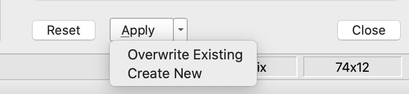
To modify the current dataframe, either click Apply or click the drop-down and select Overwrite Existing.
To create a new dataframe containing your changes, click the drop-down next to the Apply button and select Create New. A text box will appear allowing you to enter the name of the new dataframe.
Data types and formats#
The GAUSS dataframe supports four different data types:
String.
Numeric.
Category.
Date.
The Data Management pane supports type changing, as well as property management for each type.
Changing variable type#
To change a variable type select the desired type from the Type drop-down list on the Variables tab.
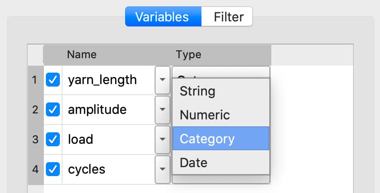
If further type-specific properties are required, a properties dialog will automatically open.
Changing categorical mappings#
Click the drop-down button to the right of the variable name and select Properties to open the Modify Column Mapping dialog.
Change a category label by double-clicking in the Renamed Label textbox next to the category label you want to change, then enter the new label name.
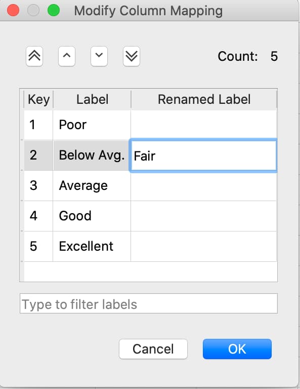
Specify a category to be the base case by selecting the Label of the category you want to be the new base case then click the double up-pointing arrow button to move the selected category to the base case.
The Category Count will be listed in the top right of the Modify Column Mapping dialog.
Specifying date formats#
If GAUSS does not automatically detect your date format, you will be asked to manually specify a date format using the Specify Date Format dialog.

Build a format string in the Date format box, using the BSD strftime specifiers, that represents your data.
If your data looked like this 03/12/2017, the correct format string would be %m/%d/%Y. The table below explains this.
Original Contents |
Description |
Type |
Format string contents |
|---|---|---|---|
03 |
A two digit month. |
Date |
|
/ |
A forward slash. |
Literal |
/ |
12 |
A two digit day. |
Date |
|
/ |
A forward slash. |
Literal |
/ |
2017 |
A four digit year. |
Date |
|
The Format Options section of this dialog contains the BSD strftime specifiers for reference. Use the Filter drop-down to filter the reference options shown.
Further Reading#
Programmatic Data Cleaning#
Missing value handling#
Counting missing variables#
The procedure dstatmt() counts missing values by variable name as part of the descriptive statistics report.
It requires only a single input indicating the source of data.
The input may be either the file name of a dataset or the name of a matrix or dataframe currently in the workspace.
// Create file name with full path
dataset = getGAUSSHome("examples/auto2.dta");

// Compute descriptive statistics and print report
// of a dataset stored on disk
call dstatmt(dataset);
-------------------------------------------------------------------------------------
Variable         Mean   Std Dev    Variance    Minimum     Maximum    Valid   Missing
-------------------------------------------------------------------------------------

make            -----     -----       -----      -----       -----       74        0
price            6165      2949     8.7e+06       3291   1.591e+04       74        0
mpg              21.3     5.786       33.47         12          41       74        0
rep78           -----     -----       -----       Poor   Excellent       69        5
headroom        2.993     0.846      0.7157        1.5           5       74        0
trunk           13.76     4.277        18.3          5          23       74        0
weight           3019     777.2    6.04e+05       1760        4840       74        0
length          187.9     22.27       495.8        142         233       74        0
turn            39.65     4.399       19.35         31          51       74        0
displacement    197.3     91.84        8434         79         425       74        0
gear_ratio      3.015    0.4563      0.2082       2.19        3.89       74        0
foreign         -----     -----       -----   Domestic     Foreign       74        0
A second optional input allows you to specify which columns to use.
// Create file name with full path
dataset = getGAUSSHome("examples/auto2.dta");

// Load data from the file
auto = loadd(dataset);

// Compute descriptive statistics and print report
// of specific variables from a dataframe
call dstatmt(auto, "price + mpg + rep78");
-------------------------------------------------------------------------------------
Variable         Mean   Std Dev    Variance    Minimum     Maximum    Valid   Missing
-------------------------------------------------------------------------------------

price            6165      2949     8.7e+06       3291   1.591e+04       74        0
mpg              21.3     5.786       33.47         12          41       74        0
rep78           -----     -----       -----       Poor   Excellent       69        5
You can count the number of missing values in a vector using counts().
// Create a column vector with 2 missing values
x = { 1, ., 3, ., 5, 6 };

// Create a missing value
m = miss();

// Count the number of missing values in the vector
n = counts(x, m);
After running the above code, n will be equal to 2.
Checking for missing values#
You can check to see if a matrix or dataframe contains any missing values with ismiss().
// Create one vector with a
// missing value and one without
a = { 1, 2, 3 };
b = { 4, ., 5 };

// Check whether the vectors contain missing values
ret_a = ismiss(a);
ret_b = ismiss(b);
After the code above, ret_a will equal 0, but ret_b will equal 1.
To find which observations contain missing values, you can use rowcontains(), indexcat(), or the dot equality operator .==. First we will load some data and then show these options.
// Create file name with full path
dataset = getGAUSSHome("examples/auto2.dta");

// Load 3 variables
auto = loadd(dataset, "mpg + price + rep78");

// Select the first 8 rows
auto = head(auto, 8);
After the above code, auto will equal:
mpg      price      rep78
 22       4099    Average
 17       4749    Average
 22       3799          .
 20       4816    Average
 15       7827       Good
 18       5788    Average
 26       4453          .
 20       5189    Average
indexcat() can tell us the row indices of a column that contains missing values.
// Create a missing value
m = miss();

// Find the indices of the rows with missing values
idx = indexcat(auto[.,"rep78"], m);
idx will now equal:
3
7
rowcontains() will return a binary vector with a 1 for each row where any element contains a missing value. Continuing with our data from above:
// Return a binary vector with a 1 for
// rows that contain a missing value
mask = rowContains(auto, miss());
mask will equal:
0
0
1
0
0
0
1
0
The dot equality operator, .== will return a binary matrix with a 1 for any element that contains a missing value. Again we will use the data loaded earlier.
// Return a binary matrix with a 1
// for any element that is a missing value
mask = auto .== miss();
mask will equal:
0    0    0
0    0    0
0    0    1
0    0    0
0    0    0
0    0    0
0    0    1
0    0    0
Removing missing values#
There are two options for removing missing values from a matrix:
packr()removes all rows from a matrix that contain any missing values.delif()removes all rows which meet a particular condition.
a = { 1 .,
      . 4,
      5 6 };

// Remove all rows with a missing value
print packr(a);
will return:
5 6
whereas:
a = { 1 .,
      . 4,
      5 6 };
 m = { . };

// Remove all rows with a missing value
// in the second column
print delif(a, a[., 2] .== m );
will only delete rows with a missing value in the second column.
. 4
5 6
Replacing missing values#
GAUSS has two functions that can be used to replace missing values:
The missrv() function replaces all missing values in a matrix with a user-specified value(s). Unique replacement values can be specified for each column.
a = { 1 .,
      . 4,
      5 6 };

// Replace all missing values with -999
print missrv(a, -999);
   1 -999
-999    4
   5    6
The impute() procedure replaces missing values in the columns of a matrix using a specified imputation method.
The procedure offers eight potential methods for imputation:
"bfill"- replaces missing values with the next valid observation (backward fill)."ffill"- replaces missing values with the most recent previous valid observation (forward fill)."mean"- replaces missing values with the mean of the column."median"- replaces missing values with the median of the column."mode"- replace missing values with the mode of the column."pmm"- replaces missing values using predictive mean matching."lrd"- replace missing values using local residual draws."predict"- replace missing values using linear regression prediction.
See the Command Reference for impute() for more details and examples.
Organization#
Sorting data#
Use sortc() to sort a matrix or dataframe in ascending order based on a certain column.
a = { 1 3 5,
      7 0 9,
      4 2 6 };

// Sort 'a' based on the second column
print sortc(a, 2);
7 0 9
4 2 6
1 3 5
Matrices and dataframes can be sorted on multiple columns using the sortmc() procedure.
a = { 1 3 5,
      7 0 9,
      4 0 6 };

// Sort 'a' based on the second and third column
print sortmc(a, 2|3);
4 0 6
7 0 9
1 3 5
Changing the order of columns#
Use the order() procedure to reorder columns in a matrix or dataframe.
// Create example matrix
X = { 9 6 2 6,
      9 8 2 1,
      3 0 2 9,
      1 0 3 0 };

// Put the 2nd and 4th columns first
X_2 = order(X, 2|4);
After the above code, X_2 will equal:
6 6 9 2
8 1 9 2
0 9 3 2
0 0 1 3
// Load some variables from a dataset
dataset = getGAUSSHome("examples/yellowstone.csv");
yellowstone = loadd(dataset, "LowtTemp + HighTemp + Visits + TotalPrecip + date($Date)");

// Reorder the dataframe so 'date' and 'visits'
// are the first two variables
yellowstone_2 = order(yellowstone, "Date" $| "Visits");
After the above code, the first four rows of yellowstone will be:
LowtTemp    HighTemp      Visits  TotalPrecip             Date
   -17.0        37.0       30621         1.09       2016/01/01
   -17.0        42.0       28091        0.770       2015/01/01
   -19.0        41.0       26778         1.28       2014/01/01
   -22.0        43.0       24699        0.610       2013/01/01
while the first four rows of yellowstone_2 look like this:
      Date     Visits    LowtTemp    HighTemp   TotalPrecip
2016/01/01      30621       -17.0        37.0          1.09
2015/01/01      28091       -17.0        42.0         0.770
2014/01/01      26778       -19.0        41.0          1.28
2013/01/01      24699       -22.0        43.0         0.610
Deleting columns#
You can delete columns from a matrix using the delcols() procedure. The columns to remove can be specified as numeric indices for matrices and dataframes:
a = { 1 3 5 7,
      7 0 9 4,
      4 2 6 2 };

// Remove the 1st and 3rd column from 'a'
print delcols(a, 1|3);
3 7
0 4
2 2
You can also use column names to delete columns from a dataframe.
// Create file name with full path
dataset = getGAUSSHome("examples/detroit.sas7bdat");

// Load  4 variables from the dataset
detroit = loadd(dataset, "unemployment + weekly_earn + hourly_earn + assault");

// Remove 2 variables from 'detroit' by name
detroit = delcols(detroit, "weekly_earn" $| "hourly_earn");

// Print the first 4 rows of 'detroit'
print detroit[1:4, .];
unemployment       assault
        11.0        306.18
         7.0        315.16
         5.2        277.53
         4.3        234.07
Deleting rows from a matrix#
Two GAUSS functions are available for deleting rows from a matrix:
delrows() deletes rows based on the specified row number.
a = { 1 2,
      3 4,
      5 6,
      7 8 };

// Remove the 2nd and 4th row of 'a'
print delrows(a, 2|4);
1 2
5 6
trimr() trims rows from either the top and bottom of a matrix.
a = { 1 2,
      3 4,
      5 6,
      7 8 };

// Trim the top row and the bottom
// 2 rows from 'a'
print trimr(a, 1, 2);
3 4
Conditionally deleting rows of data#
delif() conditionally deletes rows from a matrix, dataframe or string array based upon a logical vector.
a = { 1 2,
      3 4,
      5 6,
      7 8 };

// Remove rows where the element in the
// first column of 'a' is equal to 3
print delif(a, a[., 1] .== 3);
1 2
5 6
7 8
Conditionally selecting data#
You can conditionally select data from a matrix, dataframe, or string array using the selif() procedure.
Enter the data as the first input to selif() and the condition to be used for selecting data as the second input.
a = { 1 2,
      3 4,
      5 6,
      7 8 };

// Keep rows where the element in the second
// column of 'a' is less than or equal to 6
print selif(a, a[., 2] .<= 6);
1 2
3 4
5 6
Variable types and names#
Determining variable or column types#
Use the getColTypes() procedure to lookup the type of the variables in a dataframe. getColTypes() returns a dataframe. The table below shows the type labels and their corresponding integer values.
Value |
Label |
|---|---|
0 |
String |
1 |
Numeric |
2 |
Category |
3 |
Date |
// Load 4 variables of different types from a dataset
dataset = getGAUSSHome("examples/nba_ht_wt.xls");
nba_ht_wt = loadd(dataset, "str(Player) + cat(Pos) + Age + date($BDate, '%m/%d/%Y')");

// Check the types of each variable in 'nba_ht_wt'
print getColTypes(nba_ht_wt);
The above code will print:
    type
  String
Category
 Numeric
    Date
getColTypes() also accepts a second optional input that allows you to check only specified column types. Continuing with the data from our previous example:
// Check the types of the 2nd and 4th variables in 'nba_ht_wt'
print getColTypes(nba_ht_wt, 2|4);
will return:
    type
Category
    Date
Setting a variable type#
asdate() sets the variable type of one or more columns of a matrix or dataframe to be a date. It can also optionally set the date display format.
// Create a column of numbers which represent
// seconds since Jan 1, 1970 (Posix time)
d = {    0,
     86400,
    172800,
    259200 };

// Set the variable type of 'd' to be a date
d = dfType(d, "Date");
After the above code, d will be a date and if we print it we will see:
        X1
1970-01-01
1970-01-02
1970-01-03
1970-01-04
dftype() is the more general function. It can set columns to any of the four types: numeric, string, category or date. It also accepts an optional input specifying the indices or variable names to be checked.
// Load 3 variables of different types from a dataset
dataset = getGAUSSHome("examples/nba_ht_wt.xls");
nba = loadd(dataset, "str(player) + cat(pos) + age");
After loading the above data, the first four rows of nba will be:
         player       pos       age
 Vitor Faverani         C        25
  Avery Bradley         G        22
   Keith Bogans         G        33
Jared Sullinger         F        21
We can change the type of the second column from a categorical to a numeric variable like this:
// Set the second column to be numeric
nba = dfType(nba, "Number", "pos");
After this code, the first four rows of nba will be:
         player       pos       age
 Vitor Faverani         0        25
  Avery Bradley         2        22
   Keith Bogans         2        33
Jared Sullinger         1        21
The elements of the pos now contain only the numeric values that correspond to the string category labels. The string labels, "C", "F" and "G" have been removed.
Note
You can convert a matrix or string array to a dataframe with asdf().
Determining current variable names#
The getColNames() procedure returns the variable names assigned to columns in a matrix.
// Load all variables from a CSV file
dataset = getGAUSSHome("examples/housing.csv");
housing = loadd(dataset);

// Print the variable names from 'housing'
print getcolnames(housing);
The above code will print out the string array:
taxes
 beds
baths
  new
price
 size
In addition, it accepts an optional input specifying the indices of the columns of interest. For example, continuing with our previous example:
// Print the names of the 3rd and 5th variable name
print getcolnames(housing, 3|5);
will return:
baths
price
Setting variable names#
The setColNames() procedure changes or adds variables names to a matrix or dataframe.
// Create example matrix
X = { 1 2,
      3 4,
      5 6 };

// Assign variable names to the columns of 'X'
X = setcolnames(X, "alpha" $| "beta");

print X;
The above code will print:
alpha    beta
    1       2
    3       4
    5       6
It also accepts an optional input specifying the indices or names to be changed. For example, continuing with the example above:
// Set the second variable name from 'X' to 'gamma'
X = setcolnames(X, "gamma", 2);

print X;
The above code will print:
alpha   gamma
    1       2
    3       4
    5       6
If the data does not currently have variable names, names will be created for all columns, with default names being assigned to any columns for which user-specified names were not provided.
Managing category labels#
Extracting current category labels#
getColLabels() returns the string category labels and corresponding integer values for a categorical or string column of a dataframe.
// Create a file name with full path
dataset = getGAUSSHome("examples/auto2.dta");

// Load all variables from the dataset
auto = loadd(dataset);

// Return the string category labels and
// corresponding numeric values
{ labels, values } = getColLabels(auto, "rep78");
After running the code above:
labels =  Poor  Values = 1
          Fair           2
       Average           3
          Good           4
      Excellent          5
Alternatively, it getCategories() procedure will return the just the category labels as a GAUSS datframe:
// Get category labels as GAUSS dataframe
labels_df = getCategories(auto, "rep78");

// Print labels
labels_df;
categories
      Poor
      Fair
   Average
      Good
 Excellent
Setting category labels#
The setColLabels() procedure allows you to add or modify the labels of categorical variables.
It changes the current type of the column to a categorical variable.
// Create example matrix
X = { 1.4 0,
      1.9 2,
      2.3 1,
      0.9 2 };

labels = "low" $| "medium" $| "high";
values = { 0, 1, 2 };

// Make the second column of 'X' a
// categorical variable with the
// provided labels and values
X = setColLabels(X, labels, values, 2);

print X;
The above code will return:
 X1      X2
1.4     low
1.9    high
2.3  medium
0.9    high
Note
If a label is not provided for all key values, the unlabeled key values will be given blank labels.
Changing category labels#
The recodecatlabels() procedure changes category labels.
// Load NBA data
dataset = getGAUSSHome("examples/nba_ht_wt.xls");
nba = loadd(dataset);

// Get column labels
{ labels, values } = getColLabels(nba, "Pos");
Here are the initial category labels and order.
labels = C   values = 0
         F            1
         G            2
We can change the category labels like this:
// Specify current labels
old_labels = "C" $| "F" $| "G";

// Specify new labels to set
new_labels = "Center" $| "Forward" $| "Guard";

// Recode the old labels to the new labels
nba = recodeCatLabels(nba, old_labels, new_labels, "Pos");

// Get column labels
{ labels, values } = getColLabels(nba, "Pos");
labels =  Center   values = 0
         Forward            1
           Guard            2
As we can see above the label names have changed, but the underlying values and order are the same.
The recodecatlabels() procedure can be used to change individual labels, rather than all labels. For example, to change just one label we could have used:
// Specify current labels
old_labels = "C";

// Specify new labels to set
new_labels = "Center";

// Recode the old labels to the new labels
nba = recodeCatLabels(nba, old_labels, new_labels, "Pos");

// Get column labels
{ labels, values } = getColLabels(nba, "Pos");
Dropping category labels#
The dropCategories() procedure drops all observations of a specified category label from a dataframe and updates the category mapping. Note that this functionality is different from deleting observations using other tools like delif().
For example, consider dropping observations using delif:
// Load NBA data
dataset = getGAUSSHome("examples/nba_ht_wt.xls");
nba = loadd(dataset);

// Delete observations with 'rep78'
// equal to "Poor"
nba_no_center = delif(nba, nba[., "Pos"] .== "C");

// Get label
getCategories(nba_no_center, "Pos");
categories
         C
         F
         G
In this case, the C category label is still stored as one of the Pos labels.
To remove it when deleting labels dropCategories`() should be used.
// Drop observations and remove label from metadata
nba_no_center_2 = dropCategories(nba, "C", "Pos");

// Check 'rep78' categories
getCategories(nba_no_center_2, "Pos");
categories
         F
         G
Change the order of categories in a dataframe#
// Load dataset
dataset = getGAUSSHome("examples/yarn.xlsx");
yarn = loadd(dataset);

// Get labels and values for amplitude variable
// in yarn dataframe
{ labels_1, values_1 } = getColLabels(yarn, "amplitude");
After the above code:
labels_1 = high   values_1 = 0
            low              1
            med              2
Since Excel files do not provide labels or order for string columns, GAUSS assigns the category value based on alphabetical order. We can reorder the categories like this:
// Change the order of the category labels for the
// variable 'amplitude' in 'yarn'
yarn = reordercatlabels(yarn, "low" $| "med" $| "high", "amplitude");

// Get column labels and key values for `amplitude`
{ labels_2, values_2 } = getColLabels(yarn, "amplitude");
After the above code:
labels_2 =  low   values_2 = 0
            med              1
           high              2
Changing category base case#
The setbasecat() function provides a convenient way to set the base case for a categorical variable.
// Load the NBA dataset
dataset = getGAUSSHome("examples/nba_ht_wt.xls");
nba = loadd(dataset);

// Get column names
{ labels, values } = getColLabels(nba, "Pos");
After the above code:
labels = C   values = 0
         F            1
         G            2
You can change G to the base case like this:
// Change the `G` category to the basecase
nba = setBaseCat(nba, "G", "Pos");

// Get new labels
{ labels, values } = getColLabels(nba, "Pos");
As we can see below, the new base case, G, has been moved to the top and all the other variables have been shifted down.
labels = G   values = 0
         C            1
         F            2
Cleaning strings and category labels#
GAUSS has a comprehensive suite of tools for managing and cleaning strings.
Trimming whitespaces#
Excess whitespaces in strings and categorical variables can lead to unexpected results. To prevent this, trimming excess whitespaces should be done using one of three GAUSS procedures:
The
strtrimr()procedure strips whitespace characters from the right side.The
strtriml()procedure strips whitespace characters from the left side.The
strtrim()procedure strips whitespace characters from both the left and right side.
Example: Trimming all whitespaces
// Create string array
string names_string = { " John", "Mary ", " Jane ", "Carl" };

// Convert to string array
names_df = asDF(names_string, "First Name");

// Check names
print names_df[3];
print names_df[4];
Printing the third and fourth elements of names_df highlights the whitespaces in the First Name variable.
First Name
 Jane

First Name
      Carl
Compare this to printing the four element, which contains no whitespaces.
// Trim whitespaces
names_df = strtrim(names_df);

// Check names
print names_df[3];
print names_df[4];
First Name
      Jane

First Name
      Carl
Note
The print() function will automatically align the string array, so print header_sa will make it appear as if the leading and trailing spaces are gone. To see the spaces, we print individual elements.
Standardizing case#
Symbol names in GAUSS are not case-sensitive. For example, consider the following example of variable naming.
// Assign values to 'x'
x = 5;

// Print little x value
print "little x:" x;
little x: 5.0000000
// Assign values to 'X'
X = 10;

print "little x:" x;
little x: 10.000000
However, string and category variables, as well as variable names, are case sensitive. Because of this, inconsistent use of cases in strings and category labels can result in undesired results. For example, consider survey data with self reported location abbreviations.
// Generate states string array
st_abbreviation = "CO" $| "Co" $| "CA" $| "CA" $| "Ca" $| "Mo" $| "MO";

// Convert to dataframe
st_df = asDF(st_abbreviation, "State");

// Print observations
st_df;

// Print categories
getCategories(st_df);
Because of differences in cases, GAUSS thinks there are 6 different categories.
categories
        CA
        CO
        Ca
        Co
        MO
        Mo
Consider if we use these categories and compute a frequency count.
// Compute frequency count for 'State'
frequency(st_df, "State");
Label      Count   Total %    Cum. %
   CA          2     28.57     28.57
   CO          1     14.29     42.86
   Ca          1     14.29     57.14
   Co          1     14.29     71.43
   MO          1     14.29     85.71
   Mo          1     14.29       100
Total          7       100
To remedy this, upper() or lower() should be used to convert the state abbreviations to the same case.
// Convert to upper case
st_df = upper(st_df);

// Print 'states'
st_df;

// Compute frequency count
frequency(st_df, "State");
           State
              CO
              CO
              CA
              CA
              CA
              MO
              MO

Label      Count   Total %    Cum. %
   CA          3     42.86     42.86
   CO          2     28.57     71.43
   MO          2     28.57       100
Total          7       100
Note that upper() converts all observations of st_df to upper case and updates the label mappings.
Searching and replacing strings#
Searching and replacing is a key part of cleaning strings and categorical data. This can be done using a number of GAUSS functions:
Procedure |
Description |
|---|---|
Finds the index of one string within another string. Searches from the end to the beginning. |
|
Finds the index of one string within another string. |
|
Replaces all matches of a substring with a replacement string. |
|
Returns a 1 if a string starts with a specified pattern. |
Searching across multiple variables
The strindx() and strrindx() procedures perform element-by-element searches for substrings in string arrays. They return the starting indices of the substring or a 0 if the substring is not found.
// Create file name with full path
fname = getGAUSSHome("examples/auto2.dta");

// Load 'rep78' and 'make` variable
auto = loadd(fname, "rep78 + make");

// Preview data
head(auto);
The first five occurrences of the auto dataframe look like:
  rep78             make
Average      AMC Concord
Average        AMC Pacer
      .       AMC Spirit
Average    Buick Century
   Good    Buick Electra
Now we will search for different substrings in each separate variables.
// Find the index of "age" in 'rep78'
// and "AMC" in 'make'
idx = strindx(auto, "age"$~"AMC");

// Print the first 5 observations of 'idx'
head(idx);
The preview shows that:
In the rep78 variable, the substring
"age"starts at the fifth letter every timeAverageis observed.In the make variable, the substring
"AMC"starts at the first letter of the first three observations.
5.0000000        1.0000000
5.0000000        1.0000000
0.0000000        1.0000000
5.0000000        0.0000000
0.0000000        0.0000000
There are many uses of this. For example, suppose we want to select only the observations that contain the substring "AMC":
// Select observation if 'AMC` occurs anywhere
// in the string
amc_data = selif(auto, idx[., 2]);

// Preview data
head(amc_data);
The preview of the amc_data only prints 3 observations because only three observations remain.
  rep78             make
Average      AMC Concord
Average        AMC Pacer
      .       AMC Spirit
Searching for starting substrings
In the previous example, we search for the substring "AMC". Altenatively, startsWith() could be used to search for starting patterns.
// Load 3 variables from the dataset
fname = getGAUSSHome("examples/auto2.dta");
auto = loadd(fname, "make + price + mpg");

// Specify pattern to search for
pat = "Buick";

// Find all makes that include 'Buick'
mask = startsWith(auto[., "make"], pat);

// Select observations if the corresponding
// row of mask equals 1.
auto_buicks = selif(auto, mask);

print auto_buicks;
The code above selects all observations that start with "Buick".
         make            price              mpg
Buick Century        4816.0000        20.000000
Buick Electra        7827.0000        15.000000
Buick LeSabre        5788.0000        18.000000
   Buick Opel        4453.0000        26.000000
  Buick Regal        5189.0000        20.000000
Buick Riviera        10372.000        16.000000
Buick Skylark        4082.0000        19.000000
Regularize a string array
In this example, strreplace() is used to clean a string array that contains addresses.
// String array to be searched
str = "100 Main Ave" $|
      "112 Charles Avenue" $|
      "49 W State St" $|
      "24 Third Avenue";

// Search for string 'Avenue'
search = "Avenue";

// String to replace with
replace = "Ave";

// Build new string
new_str = strreplace(str, search, replace);
After the code above, new_str will be set to:
"100 Main Ave"
"112 Charles Ave"
"49 W State St"
"24 Third Ave"
Cleaning categorical labels
The strreplace() procedure can be used to clean categorical labels and will simultaneously updated the mapping of labels and keyvalues.
// Create 5x1 string array
states = "CA" $| "FL" $| "California" $| "California" $| "FL";

// Convert the string array to a dataframe
// with the variable name 'States'
df_states = asdf(states, "States");

// Print the dataframe
print df_states;

// Check category
getCategories(df_states);
The df_states dataframe is:
    States
        CA
        FL
California
California
        FL
And the associated categories are:
categories
        CA
California
        FL
Suppose that for the sake of our analysis, the category CA and California are treated the same. This can be corrected using the strreplace() procedure.
// Search for the "California" label
search = "California";

// Replace the "California" label with "CA"
replace = "CA";

// Call 'strreplace'
df_states = strreplace(df_states, search, replace);

// Print dataframe
print df_states;
After this, all occurrences of California have been replaced with CA.
States
    CA
    FL
    CA
    CA
    FL
Checking the categories will confirm that the keyvalues and labels have been updated.
// Get updated categories
getCategories(df_states);
As we see below, the observations that previously had the label California, have now been merged with the CA category.
categories
        CA
        FL
Extracting substrings#
The strsect() procedure extracts a substring of a string based on a specified starting point and an optional length.
// Create location string array
location = "CA, Sacramento" $| "FL Tampa" $| "SC - Charleston" $| "NC - Raleigh";

// Convert to dataframe
location_df = asDF(location, "Location");

// Print location
location_df;
The location_df variable is not consistently formatted, with the exception that the two letter state abbreviations always occurs first.
       Location
 CA, Sacramento
       FL Tampa
SC - Charleston
   NC - Raleigh
The strsect() procedure can be used to extract the state abbreviation
// Extract the state abbreviation
state = strsect(location_df, 1, 2);

// Print state
state;
Location
      CA
      FL
      SC
      NC
Splitting strings#
The strsplit() procedure can be used to split strings based on a specified separator.
// Create location string array
location = "FL, Tampa" $| "CO, Denver" $| "SC, Charleston" $| "NC, Raleigh";

// Convert to dataframe
location_df = asDF(location, "Location");

// Print preview
head(location_df);
      Location
     FL, Tampa
    CO, Denver
SC, Charleston
   NC, Raleigh
Now our Location variable contains state abbreviations and cities, separated by ",". We can use strsplit() to split the location variable into two separate columns.
// Split the location dataframe into to columns
// using ',' as a separator
location_split = strsplit(location_df, ",");

// Print location dataframe
location_split;
X1               X2
FL            Tampa
CO           Denver
SC       Charleston
NC          Raleigh
The location_split dataframe contains two columns, one that contains the state abbreviation and one that contains the city name. There are additional steps that will help further clean this data:
Rename the columns
Remove any whitespaces.
// Set column names
location_split = setColNames(location_split, "State"$|"City");

// Remove excess whitespace
location_split = strtrim(location_split);

// Print dataframe
location_split;
State             City
   FL            Tampa
   CO           Denver
   SC       Charleston
   NC          Raleigh