ridgeFit¶

Purpose¶

Fit a linear model with an L2 penalty.

Format¶

mdl = ridgeFit(y, X, lambda)¶

Parameters:

y (Nx1 vector) – The target, or dependent variable.
X (NxP matrix) – The model features, or independent variables.
lambda (Scalar, or Kx1 vector) – The L2 penalty parameter(s).

Returns:

mdl (struct) –

An instance of a ridgeModel structure. An instance named mdl will have the following members:

mdl.alpha_hat	(1 x nlambdas vector) The estimated value for the intercept for each provided lambda.
mdl.beta_hat	(P x nlambdas matrix) The estimated parameter values for each provided lambda.
mdl.mse_train	(nlambdas x 1 vector) The mean squared error for each set of parameters, computed on the training set.
mdl.lambda	(nlambdas x 1 vector) The lambda values used in the estimation.

Examples¶

Example 1: Basic Estimation and Prediction¶

new;
library gml;

/*
** Load data
*/
// Specify dataset with full path
fname = getGAUSSHome("pkgs/gml/examples/qsar_fish_toxicity.csv");

// Split data into training sets without shuffling
shuffle = "False";
{ y_train, y_test, X_train, X_test } = trainTestSplit(fname, "LC50 ~ . ", 0.7, shuffle);

// Declare 'mdl' to be an instance of a
// ridgeModel structure to hold the estimation results
struct ridgeModel mdl;

// Set lambda vector
lambda = seqm(90, 0.8, 60);

// Estimate the model with default settings
mdl = ridgeFit(y_train, X_train, lambda);

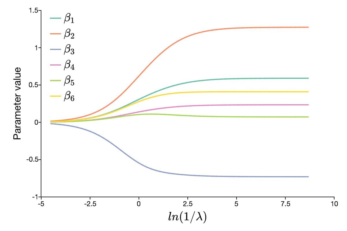
After the above code, mdl.beta_hat will be a \(6 \times 60\) matrix, where each column contains the estimates for a different lambda value. The graph below shows the path of the parameter values as the value of lambda changes.

_images/ridge-fit-example-1-beta-path.jpg

Continuing with our example, we can make test predictions like this:

/*
** Prediction for test data
*/
y_hat = lmPredict(mdl, X_test);

After the above code, y_hat will be a matrix with the same number of observations as y_test. However, it will have one column for each value of lambda used in the estimation.

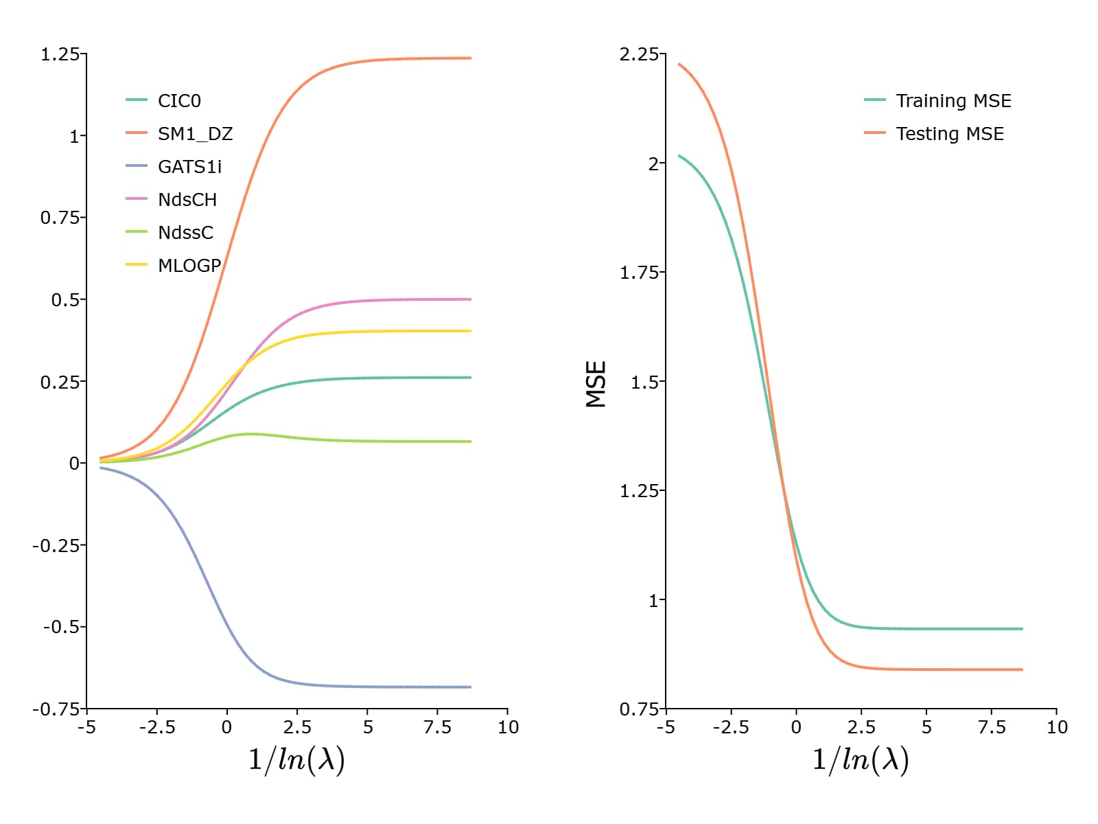
To plot the paths of the coefficients and the MSE, we can use the plotLR() function

test_mse = meanSquaredError(y_test, y_hat);

/*
** Plot results
*/
plotLR(mdl, test_mse);

This results in the following plot:

Remarks¶

Each variable (column of X) is centered to have a mean of 0 and scaled to have unit length, (i.e. the vector 2-norm of each column of X is equal to 1).